User:DukeEgr93/DSPACE2
Much of the ability to write this page came from code and examples provided by Monica Rivera - specifically the Lab 1 files for the ME 344 class as modified through Spring of 2008 by Monica Rivera and Scott Wilson.
Contents
Building a Basic Model
Building a basic Simulink model and running it on the dSPACE cards is fairly straightforward:
- Start the dSPACE ControlDesk.
- Start MATLAB - note that on a PC, the first time MATLAB is run after the PC has been turned on may take quite a bit of time to start.
- MATLAB must run a configuration script to communicate with dSPACE. In Hudson 149, the script is already set to run. If that is not the case,
dspacerc.mmust be run. That script is provided with the dSPACE card and software.
- MATLAB must run a configuration script to communicate with dSPACE. In Hudson 149, the script is already set to run. If that is not the case,
- In MATLAB, start Simulink.
- The block library should already include the dSPACE blocksets, though the individual blocks may need to be loaded. To load them, simply expand the
dSPACE RTI1104blockset. - In the Simulink Library Browser, go to File->New->Model; when the model comes up, save it inside the folder you chose when creating the experiment. For this demo, it will be called
OutputDemoModel. - The model needs to know the properties of the DSP card in order to compile the model properly. To set these properties, go to the model's window, go to Simulation->Configuration Parameters
- Solver: make sure to use a fixed-step solver; change the Fixed-step size if need be
- Hardware Implementation: choose the following:
- Device type: "Custom"
- Byte ordering: "Big Endian"
- Signed integer division rounds to: "zero"
- Once done, you can save the model.
- The block library should already include the dSPACE blocksets, though the individual blocks may need to be loaded. To load them, simply expand the
Generating Output Signals
There are several methods in Simulink for generating a signal. Most of these methods can be dynamically adjusted via the ControlDesk once the Simulink model is built and once an appropriate Layout is constructed in ControlDesk. For this documentation, a simple sinusoidal input will be used.
- Using the Simulink Library Browser, drag the following blocks into the
OutputDemoModelwindow:- Source->Sine Wave
- Sink->Out1
- This block will provide a convenient way for the ControlDesk to access the value sent to the DAC; it does not serve any other purpose in the model.
- Math Operations->Gain
- dSPACE RTI1104->DS1104 MASTER PPC->DS1104DAC_C1
- Once these blocks are in place, connect the Sine Wave to the Gain, connect the Gain to the DAC, and connect the Out1 to the wire between the Sine Wave and the Gain. Your model should resemble:
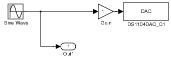
- The gain block is in place because the DAC block accepts inputs between -1 and 1 which relate to voltages between -10 and 10 V. In order for the signal you want to be properly generated by the dSPACE card, you should set the Gain block to 0.1. The Out1 block is before the gain, so it should also represent the value you want to set. Once you change the value of the gain, you may need to make the Gain block a little bigger to see the value within it. Do that, then save the model. It should now resemble:
- Each block has other options worth looking at.
- In the Sine Wave block, you can set (among other things) the Amplitude, Bias, Frequency, Phase, and Sample time. For this demonstration, leave everything as the default case except change the frequency to
2*pi*10to set it to 20\(\pi\) rad/s or 10 Hz. - The Gain block has already been set to 0.1 to compensate for the scaling factor in the DAQ block.
- The Out1 block has several parameters, none of which will be changed here.
- The DAC block has three tabs. The Unit tab which allows the user to specify which channel is being used, the Initialization tab which determines the voltage value when the dSPACE card first runs the model, and the Termination tab which determine the voltage value to set the channel at when the program terminates. This third tab should generally be checked and set to 0 volts.
- In the Sine Wave block, you can set (among other things) the Amplitude, Bias, Frequency, Phase, and Sample time. For this demonstration, leave everything as the default case except change the frequency to

That concludes perparing a model for controlling one output channel. The model will generate a signal (here with the Sine Wave block) and send it two places - an Out1 block so that ControlDesk can read it and a combination of a Gain block and a DAQ block so that the signal is scaled and sent to the appropriate digital to analog conversion channel.
Running The Model
To run the model, make sure the dSPACE ControlDesk is running. Then, in the Simulink model window, either type CTRL-B or go to Tools->Real-time Workshop->Build Model. At this point, you can watch the MATLAB Command Window print out information about compiling and loading the model. When it is finished, the compiled program will be running on the dSPACE card. Note at this point that MATLAB is not running the program - the digital signal processing card inside the dSPACE box is. In this case, if you want to see if the program is working, you need to attach the output of DACH1 to an oscilloscope or a data acquisition card running softscope.
Monitoring With ControlDesk
When the Real-Time Workshop builds a model, it generates a .SDF file containing information about the variables associated with each block. These varaibles may be monitored (and sometimes changed) in ControlDesk using a Layout. To see this, go to the ControlDesk, stop the card by clicking the red square in the navigation bar. To set things up properly:
- In the bottom of the ControlDesk, there are various tabs. Once a Simulink model is built and sent to the dSPACE cards, one of the tabs should be the SDF tab for that particular model. Go ahead and select it. The window just above the tabs should now show a "tree" with the model name at the top (using all lower-case letters) followed by Model Root, Labels, and Task Info.
- Expand the Model Root and the entries below it will be the blocks from the Simulink model, plus an extra RTI Data block that MATLAB added automatically.
- Click on the Out1 entry and the right-side window will now indicate that there is a Variable called In1 associated with it. That means ControlDesk has access to the input of that block.
- To monitor a variable, you will need to create a layout. Just above the variable explorer window is a set of four tabs. The second one, marked by a yellow rectangle above a blue square and red rectangle, is the Instrumentation tab. Select that. The window above it will indicate "No layouts open!"
- Double-click the "No layouts open!" and a new layout, layout1 will appear. This are is where you can add gauges, graphs, and other monitoring and instrumentation. To see what objects are available, go to the View menu and select Controlbars->Instrument Selector. The Instrument Selector should now be on the left side of the screen.
- For this document, you will be adding a gauge to track the current value being sent to the Out1 block. In the Virtual Instruments section of the Instrument Selector, click on the Gauge option, go into the layout, and draw a box. The size of the box will be the size of the gauge, so make it about 15 blocks wide and 15 blocks tall (based on the grid size of the layout). The layout should now resemble:
- Next you need to tell ControlDesk which variable to monitor with this gauge. The easiest way to do that is to drag the variable from the bottom right window (it should still be the In1 variable from the Out1 block) and place it on top of the gauge. The name of the gauge will change to indicate that it is now monitoring Out1/In1 - the default title for an item is the block name followed by the variable name.
- You can change gauge parameters by double-clicking the gauge. In this case, you may want to change the Range, which is in the Gauge tab, as well as the Text, which is in the Captions. Go ahead and set the range to be between -10 and 10 and set the text to "DACH1 Output" - once you have done that your layout should resemble:


You now have a gauge that is linked into your system. To use it, you will need to run the model (either by rebuilding it with CTRL-B in the Simulink model window or re-running it with the green arrow in the ControlDesk navigation bar) then tell ControlDesk to animate your layout. The main buttons are shown below:
The three buttons on the right are those associated with the layout. The left-most of those three is for "Edit" mode, which is the default case. The right-most is for "Animation" mode, which is used when the dSPACE card is running and you want to monitor or interact with variables. Go ahead and start the dSPACE card then enter Animation mode. The gauge should swing back and forth with an amplitude of 1 about 10 times per second.
10 Hz is hard to "see" on the gauge, so you will want to make some changes to your model to more clearly see how the gauge and the dSPACE card interact. Go back to the Simulink model and double-slick the Sine Wave block. Whange the amplitude to 8 and change the frequency to 2*pi*1 to make it 1 Hz. Rebuild the model with CTRL-B, then go back to the ControlDesk. Once the model has been compiled and uploaded to the card, the gauge should start making a more leisurely circuit between -8 and 8.
Interaction With ControlDesk
The Instrument Selector also has components that will allow you to use the layout to make changes to variables within a model while the program is running. For this particular model, it might be useful to adjust the amplitude while the experiment is running. To do that,
- Go to the ControlDesk and make sure the "Edit mode" is selected (the left-most of the mode buttons).
- Within the Instrument Selector, go to Virtual Instruments and click on NumericInput. Then draw a box inside the layout that is to the right of and approximately as large as the gauge from before. The layout show now resemble:
- To link this NumericInput with a particular variable, go to the bottom of the ControlDesk and make sure the SDF tab for this particular model is still selected, then in the right window, expand the Model Root and choose the Sine Wave block - there will be five variables. You can now drag the Aplitude variable on top of the NumericInput block to link them together. As before, the title will change to Sine Wave / Amplitude to reflect the block and variable within that block. If you want to change the caption, simple double-click the NumericInput box and change the Text in the Captions block. In the example below, the default is kept:
- Now re-run or re-build the model and switch into Animation Mode. The gauge should still be tracing back and forth between -8 and +8 at 1 Hz. The NumericInput box should indicate a value of 8.
- Change the value inside the NumericInput box to 4 and hit return. You should see the gauge now has a smaller oscillation, indicating your having changed the value of the amplitude of the sine wave. You can now control variables within blocks of your model while the experiment is running!


At this stage, it would be easy to add another NumericInput box, link it to the frequency of the Sine Wave block, and have more control over the Sine Wave. The following layout does just that:

One problem here, though, concerns units. The Simulink block uses radians/s for the frequency, but it may be most convenient to use Hz. The Virtual Instruments are capable of doing just that kind of conversion. Double-click on the Sine Wave/Frequency box and pick the Value Conversion tab. Since we want to display the source value from Simulink divided by 2\(\pi\), enter x/6.28319 in the Forward box. When you hit the tab key, ControlDesk will automatically fill in the Backward conversion function.
When you go back to the animation, the NumericInput block will now display (and set) the frequency in Hz:

Adding Measurements
Most models uploaded to dSPACE will need to both set voltages (as is done above) and read voltages. The dSPACE RTI1104 blockset has two different blocks for performing this task. The reason for having two different blocks is how the analog-to-digital part of the card is configured. The first four channels - ADCH1 through ADCH4 - are part of a multiplexed set of ADC channels, each of which has 16-bit resolution. The next four channels - ADCH5 through ADCH8 - are independent 12-bit inputs. In all cases, the voltage range is from -10 V to +10 V. The multiplexed group of measurements can be accessed from the MUX ADC block (labeled DS1104MUX_ADC in the block library) while individual measurements (channels 5 through 8) can each be accessed using an ADC block (labeled DS1104ADC_C5 in the block library). Note that if multiple channels are specified in the MUX ADC, the output from that block will contain multiple channels; a demultiplexer block (DEMUX) from the Signal Routing block set can split the signals up into individual channels.
It is also important to recognize that the MUX ADC and ADC blocks have the same gain issue that the DAC blocks have; that is, when voltages are measured between -10 and 10 V, the ADC signal is reported between -1 and 1. Therefore, to get output signals that match the voltage, a gain of 10 is required between the ADC block and the Out block.
The following will demonstrate how to take four different measurements - two using the multiplexed block and two using individual blocks. Starting with the model produced above:

Drag the MUX ADC block and two ADC blocks from the dSPACE RTI1104->DS1104 MASTER PPC set, a Demux block from the Signal Routing set, four Gain blocks from the Math Operations set, and four Out1 blocks from the Ports & Subsystems set. Note that MATLAB will automatically change the Out blocks to Out2, Out3, etc. as you add them; the same is true for the Gain blocks. The ADC block, however, will get an underline in front of its name. After dragging the blocks in, your model might resemble:

First, you will need to specify which channels to read from the MUX ADC. Double click that block and select any two of the four channels. The output stream from the block will have the data from both channels on it, in numerical order. For example, choosing channels 2 and 4 would bean the first data set is from channel 2 and the second datra set is from channel 4.
Next, you will need to change the channels in the ADC blocks. Assuming you want to measure channels 5 and 6, you only need to change the second (bottom) block. Double click on it and set it to read channel 6. When you change the channel, the label on the block will automatically change.
Finally, change each of the new Gain blocks to have gains of 10. That will make sure the signal being reported through the Out blocks is a measurement of the voltage.
Now that the blocks are set, you can connect them to their outputs. Note that you need to first connect the MUX ADC to the Demux block to split the data stream into two channels, then each of those two channels can go to a Gain block and finally an Out block. Once connected, your model should resemble:

To see these measurements in the ControlDesk, you will need to build the model. Make sure MATLAB's Current Directory is the same as the directory in which the model is saved, then build the model (CTRL-B).
Once MATLAB has finished building the model, you should have access to the SDF file in the ControlDesk. You can thus create some more virtual instruments and drag the new output variables to them. In the following example, there are four new displays, each set to read a different value:

Common Issues
- Make sure MATLAB's Current Directory, as indicated near the top of the MATLAB window, is the same as the directory in which your Simulink model is saved before building a model. The built model files will go in MATLAB's Current Directory, regardless of where the .mdl file is; consequently, ControlDesk will be passed a .sdf file from MATLAB's Current Directory, not necessarily the folder the .mdl file is stored. The whole process goes much more smoothly if the Current Directory is set correctly!
- Be sure to save your model before building it. The build process alone does not save the .mdl file!
Documentation
- To take a "picture" of a model, use MATLAB's
printcommand. For example, to print out a color EPS file of the model in MyModel.mdl to a file called ThePrintout.eps, use the code:
print -depsc -sMyModel ThePrintout.eps
- Note that the model must be open for MATLAB to do this. Also, the file will go in the Current Directory, regardless of where the .mdl file is saved, so make sure the Current Directory is where you want the file to go.
Specifications
The following are specifically for the dSPACE 1104 cards:
- ADC1 through ADC4 are multiplexed 16-bit ±10 V converters with approximately 1 MΩ for an input impedance
- ADC5 through ADC8 are independent 12-bit ±10 V converters with approximately 1 MΩ for an input impedance
- DACH1 through DACH8 are independent 16-bit ±10 V outputs with a current limit of ±5 mA