EGR 103/Spring 2018/Lab 2
Contents
- 1 Errors / Additions
- 2 Fixing Margins
- 3 Spell Checking
- 4 Typing Code
- 5 2.1 Introduction
- 6 2.2 Resources
- 7 2.3 Getting Started
- 8 2.4 Cantilever Beam Analysis
- 9 2.5 Creating the Script
- 10 2.6 Uploading PDFs
- 11 2.7 The Assignment
Errors / Additions
None so far for Spring 2018!
Fixing Margins
To fix the margins in the PDF documents produced by LaTeX, once logged into an OIT machine (login.oit.duke.edu) and type
texconfig
- Press return to continue, then in the window that comes up, arrow down to the second row, PAPER. Hit return, then arrow down to LETTER and hit return. You may need to press return to continue after some configuration files have been changed. When you get back to the colorful window, hit return to EXIT.
Spell Checking
To check spelling in emacs:
- Go to the Tools menu, hover over the Spell Checking item, and select Spell-Check Buffer
- See Checking and Correcting Spelling for more information. You will mainly want to read about the possible responses for the spell checker in the list that comes after the words "Here are the valid responses:" in that web page.
Typing Code
Please note - copying code from a PDF is a bad idea. While the final code is provided for you, the purpose of this assignment is for you to carefully go through the lab handout and type in the appropriate code for yourself as you go. You will learn some MATLAB commands but, more importantly, you will learn how a code is built and tested each step along the way.
2.1 Introduction
The main purpose of this lab is to go through the process of writing a complete program to load a data set, manipulate the values, perform some analysis, and create a graph. The following is a companion piece to the lab handout itself. The sections in this guide will match those in the handout.
2.2 Resources
You will want to have a browser open with the MATLAB:Script and MATLAB:Plotting pages available to you.
2.3 Getting Started
As with last week, you will want to use the
ssh -XY netid@login.oit.duke.edu
command in MobaXterm to connect to an OIT machine.
- Follow the directions to connect,
- Be sure to change into your EGR103 directory,
- Make a
lab2folder and change into it - make sure you are in the right place! - Get the tar file and expand it,
- Make a copy of the lab sample in
lab2.tex, - Start MATLAB.
2.3.1 Preview
Read and work through this section, taking notes as you go. Type in the commands at the lettered sections to see how MATLAB responds.
2.3.2 .m Files
Read and work through this section, taking notes as you go. Make sure you understand why certain lines from the script produce results on the screen and others do not.
2.4 Cantilever Beam Analysis
Read and work through this section, taking notes as you go. Note especially the process of rearranging the equation to get displacement as a function of force based on the fact that - for this experiment - the independent variable is the force.
To see the data set, go to UNIX (i.e. the MobaXterm window) and type
more Cantilever.dat
You will see an 8x2 array of data. Click Expand below to see the values here.
0.000000        0.005211
0.113510002     0.158707
0.227279999     0.31399
0.340790009     0.474619
0.455809998     0.636769
0.569320007     0.77989
0.683630005     0.936634
0.797140015     0.999986
The first column of numbers is the amount of mass in kg placed on the end of the beam - for this experiment, it ranged from 0 to about 0.8 kg (i.e. about 8 N). The second column of numbers is the displacement measured in inches, because that is what the device I used measured in. You should always take data in the original units of the device; you can convert it later.
Typically, data sets should have descriptions such as the items in the data set, units, perhaps the equipment and the person who took the measurements. For this week, however, I wanted to give you a rectangular array of data that MATLAB can easily load.
2.5 Creating the Script
Note when you open a second scripts that there are tabs in the editing window; you can choose which one to make active by clicking its tab. Be careful not to accidentally click the part of the tab that closes that tab (the X).
2.5.1 Lab Manual Syntax
For this lab, there will be several times you will simply type some items into the command window to see what they do before actually adding codes to the script. Command line only items are surrounded by a box whereas code that goes in the script has a shadowbox.
2.5.2 Comments
While you are not explicitly required to include comments in your labs -- other than the header and community standard information at the top = comments are a great way to tell yourself and your TAs what you meant to do with particular chunks of code. Also, note that a line starting with %% will set off a section in the editor window. It will have no effect on the way the program runs, just what it looks like in your editing window.
2.5.3 Initializing the Workspace
Read and work through this section, taking notes as you go; note that there are several items you will simply be typing into the command window rather than your code. The lines you will actually add from item 2. of this section are the two lines (one comment, one not) at the very end of the item 2. text. Remember - if you ever get lost on what should be in this script, the completed script is at the end of the lab handout.
2.5.4 Loading and Manipulating the Data
Read and work through this section, taking notes as you go. At the end of it, if you run your script, you should at least have matrices called Cantilever, Displacement, Force, and Mass. Type whos in MATLAB to confirm this before going forward.
2.5.5 Generating Plots
Read and work through this section, taking notes as you go. Note that the code for this is pretty far under what you've written so far; you will be filling in the blank space later, just like Taylor Swift. Too bad she can't come to the phone.
For the "During the lab, the instructor will have you create several different graphs in the command window..." this semester the instructor is going to let you navigate this part on your own. go ahead and look at the following alternate plotting commands by typing them in the command window only; at the end, there will be a plot command that you paste into your document:
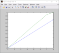
Plotting a matrix
plot(Cantilever)
Plots the matrix itself - the data points are plotted by columns with the y value coming from the data points and the x value coming from the row of the matrix. That is why there are two lines (two columns of data) and the domain goes from 1 to 8. If you
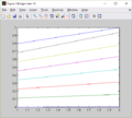
plot(Cantilever')
you are plotting a 2x8 matrix and will this see eight lines with domains from 1 to 2. Note that newer version of MATLAB will have a different color scheme.
Plot of 8x2 Matrix
Plot of 2x8 Matrix


Plotting with two inputs
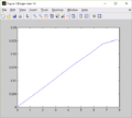
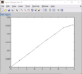
plot(Force, Displacement)
If MATLAB gets two arguments for the plot command, the first will be the independent (typically \(x\) coordinates and the second will be the dependent (typically \(y\) coordinates). The default case is to connect the dots with blue line segments. Note for this experiment that this plot would receive no credit - among other things, the axes are not labeled and there is no title. Perhaps worse than that, you have connected eight discrete experimental data points with lines. This is not appropriate for this experiment - instead, the data points should be plotted as individual points.
Plot of Displacement vs. Force

Plotting different ways
Take a look at the help file for plot in MATLAB:
help plot
and in particular the table in the middle of it. The table is also available on the Pundit page for plot at MATLAB:Plotting#The_plot_Function. The table shows that, for a particular set of independent and dependent values, you can change how MATLAB makes the plot by specifying a color, a symbol, and a line style. In the absence of a color, MATLAB will default to its built in color wheel which starts with blue in the table and works its way down - skipping white. If you give a symbol but no line style, there will be no line. If you give a line style but no symbol, no symbol will appear at each point. If you give neither, solid lines with no symbol will appear. Note that in almost all cases, the order of color, symbol, and line style does not matter - ro- will produce the same as -ro. The only case where the order matters is when it comes to specifying a dash-dot line versus trying to specify a situation where there are large dots at each point and a solid line connecting the points. Take a look at
plot(Force, Displacement, 'k-.')
versus
plot(Force, Displacement, 'k.-')
as an example.
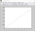
A dot-dash line
Dots with a solid line


Things to avoid
Here are a few examples to avoid:
plot(Force, Displacement, 'mp')
Uses purple pentagrams. It's adorable, though perhaps not professional.
plot(Force, Displacement, 'bh')
Using symbols that have cultural or religious meanings should be avoided unless wholly appropriate to the data set.
plot(Force, Displacement, 'k+')
The problem here isn't necessarily that the + look like crosses but rather that the data point in the bottom left corner looks like it might be the origin instead of a data point. Later, you will learn to use a command that zooms out so no point is on the figure boundary. For today, just avoid using the +.
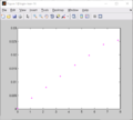
Purple pentagrams!
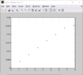
Blue Stars of David!
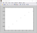
Potentially Confusing Pluses!


The right answer
For this lab, the right answer will be to use black ink and to use circles at the points with no connecting lines, so:
plot(Force, Displacement, 'ko')

2.5.6 Polynomials in MATLAB
Read and work through this section, taking notes as you go. Be sure you and your neighbor understand how MATLAB interprets polynomials and which commands use them.
2.5.7 Generate Predictions
Read and work through this section, taking notes as you go. This part creates a new set of data points based on your equation so that you can actually plot it. You will thus have your original eight data points in Force and Displaement. You will also have 100 linearly spaced values between the minimum and maximum force value in ForceModel and the 100 calculated estimates for the displacement, based on your best straight line, in DispModel.
2.5.8 Generating Plots (revisited)
Read and work through this section, taking notes as you go. This part adds the new line to your old graph.
CRITICALLY IMPORTANT PART - never put an ending on the filename of a print command in MATLAB. MATLAB will automagically add the correct extension (for us, typically .eps) if there is not one, but if you put one, MATLAB will save the file to exactly that name. It could be a disaster if, for example you give a filename like lab2.tex...Which you will never do. Because you will never put an ending on the filename of a print command in MATLAB.
You can check to see if this worked by going into your terminal window and typing:
evince RunCanPlot.eps
Note that sometimes MATLAB will not be able to display graph elements correctly - this is particularly true if Greek symbols are in your titles or labels. If you save the graph, evince should show the symbols correctly.

2.6 Uploading PDFs
You will be earning homework points for this lab by submitting a PDF version of your completed plot for the cantilever beam.
- First, you will need to convert it from an eps file to a pdf file so it is easier for the TAs to see.
In your lab2 directory, once you have created the RunCanPlot.eps file, run the command
ps2pdf RunCanPlot.eps
- See EGR_103/Uploading_Solutions
- Go through the process to actually submit what you have for your RunCanPlot.pdf document to the "Cantilever Plot" assignment.
- Have a TA confirm that they can see what you've uploaded - they will grade it right then.
2.7 The Assignment
Basically, once you get this script running perfectly, you are going to replicate it three times and change it to use three different data sets. Note: these three data sets are "cooked" - that is, I produced them; they did not come from an experiment.
2.7.1 What the .m-files Should Do
Read and work through this section, taking notes as you go.
2.7.2 The Lab Report
Read and work through this section, taking notes as you go. Note that the data sets have different numbers of points so the bottoms of the data tables will not line up. Also note that you should use the original data (masses and displacements in inches) in the tables -- do not put in the forces or the displacements in meters. You are using the latter in your calculations but you are presenting the original data sets here.
2.7.3 Processing the Lab Report
Seriously - spell check!