Difference between revisions of "EGR 224/Measurements 2"
| Line 1: | Line 1: | ||
| − | The following page provides some supplemental information for the '''Basic Electrical Measurements II''' lab for [[EGR 224|EGR 224L]]. It has been updated for Spring, | + | The following page provides some supplemental information for the '''Basic Electrical Measurements II''' lab for [[EGR 224|EGR 224L]]. It has been updated for Spring, 2018. |
== Clarifications / Troubleshooting == | == Clarifications / Troubleshooting == | ||
| Line 28: | Line 28: | ||
Click on the pictures above to make them larger. | Click on the pictures above to make them larger. | ||
| − | + | == Plotting == | |
| + | For your plots, the total voltage should be a solid (dark) red line, the capacitor voltage should be a dash-dot (dark) blue line, and the resistor voltage should be a dashed (dark) green line. Here are some examples of how to do that in Maple, (less efficiently) in all versions of MATLAB, and (more efficiently) in newer versions of MATLAB, plotting t^2, t, and t^2-t: | ||
| + | === Maple === | ||
| + | <source lang=maple> | ||
| + | plot([t^2, t, t^2-t], t = 0 .. 3, linestyle = [1, 4, 3], legend = ['Total', 'vC', 'vR'], title = 'Title') | ||
| + | </source> | ||
| + | === All MATLAB === | ||
| + | The following set the line widths to 1 for each plot and then sets the color based on a value for red, green, and blue -- these need to be between 0 and 1 for each component. [0.5 0 0] is thus dark red, [0 0 0.5] is dark blue, and [0 0.5 0] is dark green. These need to be darker than MATLAB's defaults because, for example, the default green is too light. | ||
| + | <source lang=matlab> | ||
| + | Time = linspace(0, 3, 100); | ||
| + | plot(Time, Time.^2, 'k-', 'LineW', 1, 'Color', [0.5 0 0]) | ||
| + | hold on | ||
| + | plot(Time, Time, 'k-.', 'LineW', 1, 'Color', [0 0 0.5]) | ||
| + | plot(Time, Time.^2-Time, 'k--', 'LineW', 1, 'Color', [0 0.5 0]) | ||
| + | hold off | ||
| + | legend('Total', 'v_{C}', 'v_{R}', 'location', 'best') | ||
| + | </source> | ||
| + | ===Newer MATLAB=== | ||
| + | For MATLAB 2014b or newer, there is a more efficient way to use the plot object to do the same work: | ||
| + | <source lang=matlab> | ||
| + | Time = linspace(0, 3, 100); | ||
| + | p=plot(Time, Time.^2, 'k-', Time, Time, 'k-.', Time, Time.^2-Time, 'k--'); | ||
| + | p(1).Color = [0.5 0 0]; p(1).LineWidth = 1; | ||
| + | p(2).Color = [0 0 0.5]; p(2).LineWidth = 1; | ||
| + | p(3).Color = [0 0.5 0]; p(3).LineWidth = 1; | ||
| + | legend('Total', 'v_{C}', 'v_{R}', 'location', 'best') | ||
| + | </source> | ||
| + | The p object has information about each of the items that were plotted; you can then set them individually rather than having to have multiple plot commands. Note that Duke's UNIX system has MATLAB 2014a (so close!) so this will not work as yet on that system. | ||
[[Category:EGR 224]] | [[Category:EGR 224]] | ||
Revision as of 02:56, 20 February 2018
The following page provides some supplemental information for the Basic Electrical Measurements II lab for EGR 224L. It has been updated for Spring, 2018.
Contents
Clarifications / Troubleshooting
- If you get a "specified device not found" or something like that, try using 'Dev2' instead of 'Dev1' in the TestFunction code.
- If one of your figures looks wrong, it probably is! Be sure to have a TA check your figures so that you leave the lab with a valid data set.
Element Values
- Resistances:
- 1, 9, 17: 2.2 k\(\Omega\)
- 2, 3, 10, 11, 18, 19: 4.7 k\(\Omega\)
- 4, 5, 12, 13, 20, 21: 10 k\(\Omega\)
- 6, 14, 16, 22: 15 k\(\Omega\)
- 7, 8, 15, 23, 24: 22 k\(\Omega\)
- Capacitances
- 7, 15, 23: 2.2 \(\mu\)F
- 4, 6, 8, 12, 14, 16, 20, 22, 24: 4.7 \(\mu\)F
- 2, 5, 10, 13, 18, 21: 10 \(\mu\)F
- 1, 3, 9, 11, 17, 19: 22 \(\mu\)F
Links
- The files for this assignment can be downloaded from http://classes.pratt.duke.edu/FILES/EGR224/DAQS/ElecMeas2
Wiring Images
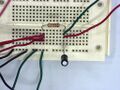
Closeup of the breadboard
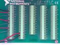
Closeup of the CB-68LP


Click on the pictures above to make them larger.
Plotting
For your plots, the total voltage should be a solid (dark) red line, the capacitor voltage should be a dash-dot (dark) blue line, and the resistor voltage should be a dashed (dark) green line. Here are some examples of how to do that in Maple, (less efficiently) in all versions of MATLAB, and (more efficiently) in newer versions of MATLAB, plotting t^2, t, and t^2-t:
Maple
plot([t^2, t, t^2-t], t = 0 .. 3, linestyle = [1, 4, 3], legend = ['Total', 'vC', 'vR'], title = 'Title')All MATLAB
The following set the line widths to 1 for each plot and then sets the color based on a value for red, green, and blue -- these need to be between 0 and 1 for each component. [0.5 0 0] is thus dark red, [0 0 0.5] is dark blue, and [0 0.5 0] is dark green. These need to be darker than MATLAB's defaults because, for example, the default green is too light.
Time = linspace(0, 3, 100);
plot(Time, Time.^2,      'k-',  'LineW', 1, 'Color', [0.5 0 0])
hold on
plot(Time, Time,         'k-.', 'LineW', 1, 'Color', [0 0 0.5])
plot(Time, Time.^2-Time, 'k--', 'LineW', 1, 'Color', [0 0.5 0])
hold off
legend('Total', 'v_{C}', 'v_{R}', 'location', 'best')
Newer MATLAB
For MATLAB 2014b or newer, there is a more efficient way to use the plot object to do the same work:
Time = linspace(0, 3, 100);
p=plot(Time, Time.^2, 'k-', Time, Time, 'k-.', Time, Time.^2-Time, 'k--');
p(1).Color = [0.5 0 0]; p(1).LineWidth = 1;
p(2).Color = [0 0 0.5]; p(2).LineWidth = 1;
p(3).Color = [0 0.5 0]; p(3).LineWidth = 1;
legend('Total', 'v_{C}', 'v_{R}', 'location', 'best')
The p object has information about each of the items that were plotted; you can then set them individually rather than having to have multiple plot commands. Note that Duke's UNIX system has MATLAB 2014a (so close!) so this will not work as yet on that system.