MATLAB:Logical Masks
Introduction
Many times, you will see functions that are written in some kind of piecewise fashion. That is, depending upon that value of the input argument, the output argument may be calculated in one of several different ways. In these cases, you can use MATLAB's logical and relational arguments to create logical masks - matrices containing either 0's or 1's - to help determine the appropriate calculation to perform to determines the values in a matrix.
Example 1: Piecewise Constant
Take for example GPA as a function of numerical grade (assume \(\pm\) do not exist for the moment...). The mathematical statement of GPA might be:
\( \mbox{GPA}(\mbox{Grade})&=\left\{ \begin{array}{rl} \mbox{Grade}\geq 90 & 4.0\\ 80\leq\mbox{Grade} ~\&~ \mbox{Grade}<90 & 3.0\\ 70\leq\mbox{Grade} ~\&~ \mbox{Grade}<80 & 2.0\\ 60\leq\mbox{Grade} ~\&~ \mbox{Grade}<70 & 1.0\\ \mbox{Grade}<60 & 0.0 \end{array} \right. \)
If you want to write this table as a function that can accept multiple
inputs at once, you really should not use an if-tree
(because if-trees can only run one program segment for the entire matrix) or a
for loop (because for loops are slower and more complex
for this particular situation).
Instead, use MATLAB's ability to create logical masks. Look
at the following code:
Grade=linspace(0, 100, 1000);
MaskForA = Grade>=90;
The variable MaskForA will be the same size of the Grade
variable, and will contain only 0's and 1's -- 0 when the logical
expression is false and 1 when it is true. Given that, you can use
this in conjunction with the function for an "A" grade to start
building the GPA variable:
Grade=linspace(0, 100, 1000);
MaskForA = Grade>=90;
FunctionForA = 4.0;
GPA = MaskForA.*FunctionForA;
At the end of this code, the GPA variable will contain a 4.0
wherever the logical mask MaskForA was a 1 and it will contain a
0.0 wherever the logical mask was a 0. All that is required is to
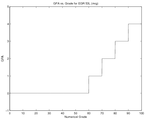
extend this to the rest of the possible GPA's - the full code is in the section below, along with an image of the graph it will create. Note the use of the continuation ... to write the commands in the same
visual way the function definition is written - this is not required, but
does make the code easier to interpret.
Also, the axes of the graph have been changed using the axis
command so that the graph is not directly on top of the border of the
plot. Without this change, the "A" portion of the graph would be
hidden by the top edge of the figure boundary.
|
Code: Grade=linspace(0, 100, 1000);
MaskForA = Grade>=90;
FunctionForA = 4.0;
MaskForB = 80<=Grade & Grade<90;
FunctionForB = 3.0;
MaskForC = 70<=Grade & Grade<80;
FunctionForC = 2.0;
MaskForD = 60<=Grade & Grade<70;
FunctionForD = 1.0;
MaskForF = Grade<60;
FunctionForF = 0.0;
GPA = ...
MaskForA.*FunctionForA + ...
MaskForB.*FunctionForB + ...
MaskForC.*FunctionForC + ...
MaskForD.*FunctionForD + ...
MaskForF.*FunctionForF;
plot(Grade, GPA)
axis([0 100 -1 5])
xlabel('Numerical Grade')
ylabel('GPA')
title('GPA vs. Grade for EGR 53L (mrg)')
print -deps GPAPlot
|
