Difference between revisions of "EGR 103/Fall 2017/Lab 6"
| Line 58: | Line 58: | ||
=== 5.4.4 Palm 5.33 === | === 5.4.4 Palm 5.33 === | ||
| − | The main programming concepts here are creating contour plots and imagesc plots. More information on the former can be found at [[MATLAB:Contour_Plots]] | + | The main programming concepts here are creating contour plots and imagesc plots. More information on the former can be found at [[MATLAB:Contour_Plots]]. The temperatures are in degrees Celsius and the distances are in meters. |
=== 5.4.6 Palm 4.28 === | === 5.4.6 Palm 4.28 === | ||
Revision as of 17:03, 17 October 2017
The following document is meant as an outline of what is covered in this assignment.
Contents
Typographical Errors
None yet!
Specific Problems
Chapra Problem 4.1
The primary goals here are to re-use an iterative solver with a different iterator and to present the information in a table generated for LaTeX by MATLAB.
- The code on page 94 of the Chapra book, in Figure 4.2, is incredibly useful and important. You will need to have it memorized eventually, but for now focus on understanding how it does what it does.
- One difference between your code and the code in the book is that your original
solwill be set equal to the first input, calledainstead ofxin your code. This will happen on the line under the comment% initialization - One more difference will be on the line where
solgets updated. Make sure you understand where and how the update is happening in the original code with the original iterator, then re-write it for your iterator. - The page on MATLAB:LaTeX_Table_Writer really will be helpful; note that the
RunDivAvg.mcode already has comments where you need to make changes. - The section on MATLAB:LaTeX_Table_Writer#Saving_to_a_File will explain what the
fopenandfclosefunctions, as wellFIDvariable, do. - Here is the original
RunDivAvg
%% Initialize the workspace
clear; format short e
%% Set up lists of parameters
a = [ones(1,4)*16, ...
     ones(1,4)*160, ...
     ones(1,4)*1600, ...
     ones(1,4)*16000, ...
     ones(1,4)*160000];
es = repmat([1e-2 1e-2 1e-8 1e-8], 1, 5);
maxit = repmat([5 12], 1, 10);
%% Run loop and store 20 sets of results
for k=1:20
    [fx(k), ea(k), iter(k)] = DivAvg(a(k), es(k), maxit(k));
end
%% Open file for writing
FID = fopen('DivAvgTable.tex', 'w');
%% Write the table to a file
% print the tabular line and a newline
fprintf(FID, '\n\\begin{tabular}{|ccc|ccc|}\\hline \n');
% print the table headers and a horizontal line then a newline
fprintf(FID, '$a$ & $\\epsilon_s$ & maxit & $\\sqrt{a}$ & $\\epsilon_a$ & iter\\\\ \\hline \n');
for k=1:20
    % print a line of the table - but no newline!
    %%% YOUR CODE HERE

    % print a horizontal line every 4 row
    if 0 %%% YOUR LOGIC REPLACES THE 0 HERE
        fprintf(FID, '\\hline ');
    end
    % print a newline
    fprintf(FID, '\n');
end
fprintf(FID, '\\end{tabular}\n');
%% Close the file
fclose(FID);
Palm Figure 6.1-2, p. 265
The main goals here are to learn how to put italics and math in labels and titles and how to put text on a plot.
- Information on how to labels axes and the title, including using italics: MATLAB:Plotting#General_Plotting_Tips
- Information on putting text on a plot is at: MATLAB:Plotting#Putting_Text_on_a_Plot
- Information for setting the limits and tick locations is at MATLAB:Plotting#Setting_Limits_and_Tick_Locations
5.4.4 Palm 5.33
The main programming concepts here are creating contour plots and imagesc plots. More information on the former can be found at MATLAB:Contour_Plots. The temperatures are in degrees Celsius and the distances are in meters.
5.4.6 Palm 4.28
This problem expands on making surface plots to using 2-D matrices to solve optimization problems. MATLAB:Plotting_Surfaces and MATLAB:Contour_Plots will be useful in making the plots. The section MATLAB:Plotting_Surfaces#Finding_Minima_and_Maxima_in_2-D will be especially helpful in terms of finding the best location for the distribution center.
When testing your code, best bet is to write code to first calculate the distances between one customer and your grid of points. Make a surface plot of that to see if the distance calculations are 0 at the customer and increase radially from there. You can make a one customer data file by running MakeCustomers and entering 1 as the NetID. Then try to figure out how to get the cost function for just that one customer and plot it. With one customer, you can also try to get the rest of the plots as well as the customer map working. You can also find the ideal location and its cost - it should be where the customer is (which is (-22, 4) using MakeCustomersfor one customer) and the cost should be free.
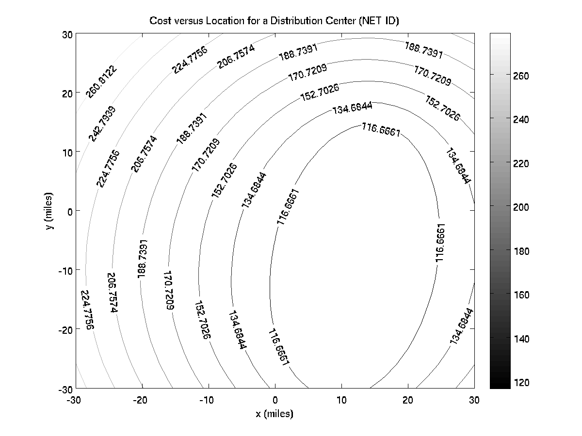
Once you have figured out one customer, put some thought into the work you need to do for two customers - how are you going to get and store the locations and volumes? What's the best way to get the total cost at each location for two customers? For N customers? Note that with two customers the best location will be at (12, -8) because that grid point happens to be closest to the straight line between the customer at (9,-28) and the customer at (15,11); since the two customers have equal volumes, the optimal location is anywhere along that straight line. You can see this in the contour plot:

Also, Douglas Adams wrote funny books.