Python:Plotting/Subplots
There are some examples in the main Python:Plotting page showing how to set up subplots within a figure window. Here are some more examples, where each example assumes
import numpy as np
import matplotlib.pyplot as plt
has already run. Note: once you have your subplots created, labeled, and titled, you definitely want to run
fig.tight_layout()
before saving; Python does not do a great job with leaving space for things with subplots.
Contents
Basics
There are three different ways to create subplots:
- fig.add_subplot() needs you to create the figure handle first (probably with
fig=plt.figure()and then you can use that figure variable to create one set of axes within an array of axes.- The three main arguments for
fig.add_subplot(nrows, ncols, index)will establish how many rows and columns you want to break the figure into and then which one of those subplots you want to work with. This method can be especially useful if you want to build a figure with several non-overlapping subplots of different shapes - more on that below.
- The three main arguments for
- plt.subplots() allows you to create the figure and the axes handles at the same time.
- The two main arguments for
plt.subplots(nrows, ncols)will establish how many rows and columns you want to break the figure into. It will return a figure handle as well an array of axes handles (1D array if creating a single column or row, 2D array if there is more than one row and more than one column). This is useful if you have an array of axes and you are planning to use all of them. You can also give the typical figure keyword arguments such asnum=1, clear=True
- The two main arguments for
- fig.subplots() needs you to create the figure handle first (probably with
fig=plt.figure()and then you can use that figure variable to create an entire array of axes.- The two main arguments for
fig.subplots(nrows, ncols)will establish how many rows and columns you want to break the figure into. It will return an array of axes handles (1D array if creating a single column or row, 2D array if there is more than one row and more than one column). This is useful if you have an array of axes and you are planning to use all of them. The only real difference between this version and the figure based one above is that this one will accept keyword arguments to be passed to the axes rather than to the figure. This will become important when creating 3D plots.
- The two main arguments for
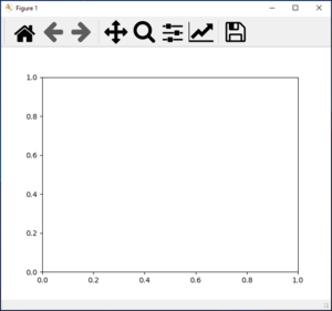
Single Subplot For The Whole Figure
Using fig.add_subplot()
fig = plt.figure(num=1, clear=True)
ax = fig.add_subplot(1, 1, 1)
Using plt.subplots()
The default for this command is to make a single subplot, so there is no row or column information necesary.
fig, ax = plt.subplots(num=1, clear=True)
Using fig.subplots()
The default for this command is to make a single subplot, so there is no row or column information necesary.
fig = plt.figure(num=1, clear=True)
ax = fig.subplots()
Single Row or Column of Subplots
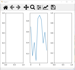
The examples below will show how to set up and access a single row or column of subplots. Imagine you want to have a single row with three columns of subplots. You can either set up three variables, one to access each set of axes, or you can set up a single variable that stores all four axes handles. In the latter case, the variable storing the axes will be a 1D array of handles, so you will access each one with a single index value.
Using fig.add_subplot()
This version requires that you set each up individually. This can be useful if each set of axes has different characteristics (for instance, if some have 3D graphs and others do not).
fig = plt.figure(num=1, clear=True)
ax1 = fig.add_subplot(1, 3, 1)
ax2 = fig.add_subplot(1, 3, 2)
ax3 = fig.add_subplot(1, 3, 3)
If you want to plot 10 uniformly distributed random numbers in the second subplot, you would use:
ax2.plot(np.random.uniform(size=10))
Using plt.subplots()
The first two positional arguments are the number of rows and the number of columns of plots to make. In this case, the ax variable will be a 1D array with four elements - one per subplot.
fig, ax = plt.subplots(1, 3, num=1, clear=True)
If you want to plot 10 uniformly distributed random numbers in the second subplot, you would use:
ax[1].plot(np.random.uniform(size=10))
Using fig.subplots()
The first two positional arguments are the number of rows and the number of columns of plots to make. In this case, the ax variable will be a 1D array with four elements - one per subplot.
fig = plt.figure(num=1, clear=True)
ax = fig.subplots(1, 3)
If you want to plot 10 uniformly distributed random numbers in the second subplot, you would use:
ax[1].plot(np.random.uniform(size=10))
If you have a single column of subplots and you want all of them to have the same $$x$$ axis (basically, to have a single labeled $$x$$ axis showing on the bottom plot), you can use code similar to that below (example shows three rows of plots):
fig, ax = plt.subplots(3, 1, num=1, clear=True, sharex=True)
# plot things
ax[2].set(xlabel="label")
or
fig = plt.figure(num=1, clear=True)
ax = fig.subplots(3, 1, sharex=True)
# plot things
ax[2].set(xlabel="label")
Multiple Rows and Columns of Subplots
If you want more than one row and more than one column of subplots, you can also create them three different ways. The add_subplot command will still create one at a time while the two different subplots() commands will now create 2D arrays of handles, meaning you will need to give two index values to access a plot.
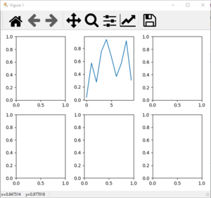
Imagine you want to have two rows with three columns of subplots. You can either set up six variables, one to access each axes, or you can set up a single 2D array that stores all six axes handles.
Using fig.add_subplot()
This version requires that you set each up individually. This can be useful if each set of axes has different characteristics (for instance, if some have 3D graphs and others do not) but starts to get tedious with a large number of subplots. Note that the subplot index (the third argument) starts with 1 in the top left corner, counts up left to right, and then goes to the next row (similar to a phone dial).
fig = plt.figure(num=1, clear=True)
ax1 = fig.add_subplot(2, 3, 1)
ax2 = fig.add_subplot(2, 3, 2)
ax3 = fig.add_subplot(2, 3, 3)
ax4 = fig.add_subplot(2, 3, 4)
ax5 = fig.add_subplot(2, 3, 5)
ax6 = fig.add_subplot(2, 3, 6)
If you want to plot 10 uniformly distributed random numbers in the second subplot, you would use:
ax2.plot(np.random.uniform(size=10))
Using plt.subplots()
The first two positional arguments are the number of rows and the number of columns of plots to make. In this case, the ax variable will be a 2D array with six elements - one per subplot.
fig, ax = plt.subplots(2, 3, num=1, clear=True)
If you want to plot 10 uniformly distributed random numbers in the second subplot (top row, middle column), you would use:
ax[0][1].plot(np.random.uniform(size=10))
Using fig.subplots()
The first two positional arguments are the number of rows and the number of columns of plots to make. In this case, the ax variable will be a 2D array with six elements - one per subplot.
fig = plt.figure(num=1, clear=True)
ax = fig.subplots(2, 3)
If you want to plot 10 uniformly distributed random numbers in the second subplot (top row, middle column), you would use:
ax[0][1].plot(np.random.uniform(size=10))
Mondrian Subplots
If you want to build a figure out of a series of rectangular subplots that are of differing sizes, you can do that with the fig.add_subplot() command. The key is that no two subplots can take up any of the same space.
Also, each subplot has to be a single location that you can create in an array of subplots - you cannot have a subplot that takes up 2/3rds of the total width of the screen, for instance.
Here are some examples of how this works:
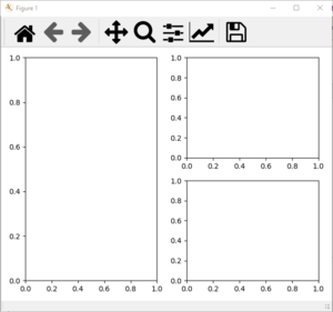
One Left, Two Right
fig  = plt.figure(num=1, clear=True)
axL  = fig.add_subplot(1, 2, 1)
axR1 = fig.add_subplot(2, 2, 2)
axR2 = fig.add_subplot(2, 2, 4)
Notice that for axL the arguments split the whole figure into one row of two columns and picked the first (left one), then for the axR1 and axR2 lines the arguments split the figure into two rows of two columns and picked the top right and bottom right. These three do not overlap at all, so the figure can support these three shapes together.
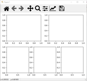
Two Top, Three Bottom
fig  = plt.figure(num=1, clear=True)
axTL = fig.add_subplot(2, 2, 1)
axTR = fig.add_subplot(2, 2, 2)
axB1 = fig.add_subplot(2, 3, 4)
axB2 = fig.add_subplot(2, 3, 5)
axB3 = fig.add_subplot(2, 3, 6)
Note that while this will work, fig.tight_layout() no longer works - the warning is that "number of columns in subplot specifications must be multiples of one another."
