EGR 103/Spring 2017/Lab 5
This page is meant to serve as the basis for a self-guided tour of the various parts of Lab 5 for EGR 103. It will include relevant links and example for each problem.
Typographical Errors
None yet!
5.4 Assignment
5.4.1 Palm 5.3(a)
Main thing to note here is that as you zoom in on the roots, the resolution gets progressively worse. Once you get a general idea of the root location, your zoomed-in plot may reveal that you aren't as close as you think you are. You might need to iterate with a few guesses of where the root is before getting it to three decimal places.
Also note that you can break the figure window up into rectangles of different sizes as long as no rectangle overlaps another. In this case, there are two columns of subplots; the left one is broken into two rows and the right one into three.
5.4.2 Palm 5.21/6.7
Just three different ways of looking at a data set!
5.4.3 Chapra 3.9
The core of this problem is to learn how to make a surface plot with contours. MATLAB:Plotting_Surfaces contains a great deal of information about this process. The meshgrid command is especially important.
5.4.4 Palm 5.33
The main programming concepts here are creating contour plots and imagesc plots. More information on the former can be found at MATLAB:Contour_Plots
5.4.5 Palm 5.36
The main programming concepts here are using meshc and surfc. Check to make sure you calculated the radii correctly -- the high potential should be closer to the larger charge.
5.4.6 Palm 4.28
This problem expands on making surface plots to using 2-D matrices to solve optimization problems. MATLAB:Plotting_Surfaces and MATLAB:Contour_Plots will be useful in making the plots. The section MATLAB:Plotting_Surfaces#Finding_Minima_and_Maxima_in_2-D will be especially helpful in terms of finding the best location for the distribution center.
When testing your code, best bet is to write code to first calculate the distances between one customer and your grid of points. Make a surface plot of that to see if the distance calculations are 0 at the customer and increase radially from there. You can make a one customer data file by running MakeCustomers and entering 1 as the NetID. Then try to figure out how to get the cost function for just that one customer and plot it. With one customer, you can also try to get the rest of the plots as well as the customer map working. You can also find the ideal location and its cost - it should be where the customer is (which is (-22, 4) using MakeCustomersfor one customer) and the cost should be free.
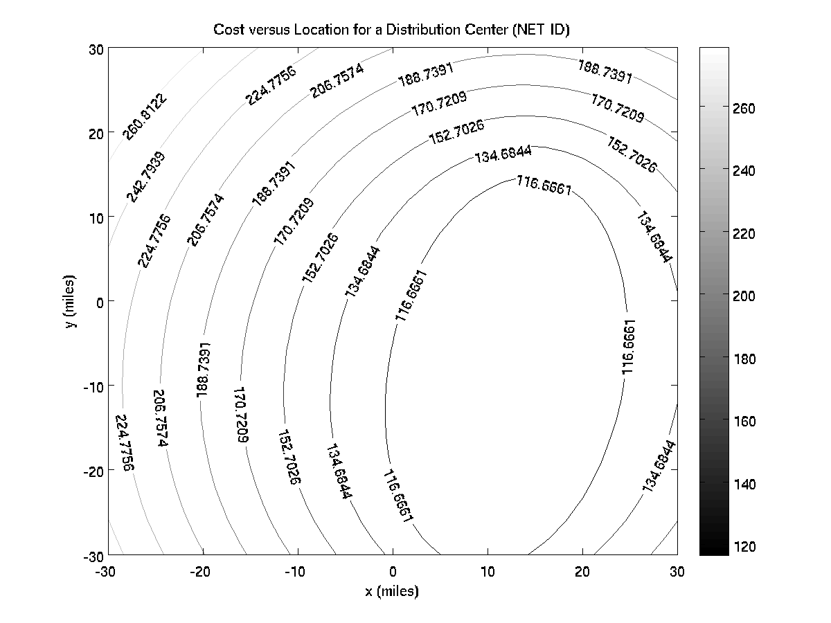
Once you have figured out one customer, put some thought into the work you need to do for two customers - how are you going to get and store the locations and volumes? What's the best way to get the total cost at each location for two customers? For N customers? Note that with two customers the best location will be at (12, -8) because that grid point happens to be closest to the straight line between the customer at (9,-28) and the customer at (15,11); since the two customers have equal volumes, the optimal location is anywhere along that straight line. You can see this in the contour plot:

Also, Douglas Adams wrote funny books.