Python:Ordinary Differential Equations/Examples

The following examples show different ways of setting up and solving initial value problems in Python. It is part of the page on Ordinary Differential Equations in Python and is very much based on MATLAB:Ordinary Differential Equations/Examples.

Examples

Note - each example began with the Templates provided at this web site. Some comments have been removed from the templates to conserve space while some comments may have been added to provide a clearer explanation of the process for a particular example. They all assume a file called ode_helpers.py that contains the code is in the same folder as the example codes:

import numpy as np
import matplotlib.pyplot as plt

def state_plotter(times, states, fig_num):
    num_states = np.shape(states)[0]
    num_cols = int(np.ceil(np.sqrt(num_states)))
    num_rows = int(np.ceil(num_states / num_cols))
    f, ax = plt.subplots(num_rows, num_cols, num=fig_num, clear=True,
                         squeeze=False)
    for n in range(num_states):
        row = n // num_cols
        col = n % num_cols
        ax[row][col].plot(times, states[n], 'k.:')
        ax[row][col].set(xlabel='Time',
                         ylabel='$y_{:0.0f}(t)$'.format(n),
                         title='$y_{:0.0f}(t)$ vs. Time'.format(n))
        f.tight_layout()
    for n in range(num_states, num_rows * num_cols):
        f.delaxes(ax[n // num_cols][n % num_cols])

Constant Rate of Change

Result using constant rate of change.

If the dependent variable has a constant rate of change:

\( \begin{align} \frac{dy}{dt}=C\end{align} \)

where \(C\) is some constant, you can provide the differential equation in the f function and then calculate answers using this model with the code below. The code assumes there are 100 evenly spaced times between 0 and 10, the initial value of \(y\) is 6, and the rate of change is 1.2:

# %% Imports
import numpy as np
import matplotlib.pyplot as plt
from scipy.integrate import solve_ivp
from ode_helpers import state_plotter

# %% Define independent function and derivative function
def f(t, y, c):
    dydt = [c[0]]
    return dydt

# %% Define time spans, initial values, and constants
tspan = np.linspace(0, 10, 100)
yinit = [6]
c = [1.2]

# %% Solve differential equation
sol = solve_ivp(lambda t, y: f(t, y, c), 
                [tspan[0], tspan[-1]], yinit, t_eval=tspan)

# %% Plot states
state_plotter(sol.t, sol.y, 1)

Time-dependent Rate of Change

Result using time-varying rate of change

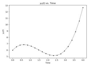
If the dependent variable's rate of change is some function of time, this can be easily coded. For example, if the differential equation is some quadratic function given as:

\( \begin{align} \frac{dy}{dt}&=\alpha t^2+\beta t+\gamma \end{align} \)

then the function providing the values of the derivative may be written using np.polyval. You could calculate answers using this model with the following code; it assumes there are 20 evenly spaced times between 0 and 4, the initial value of \(y\) is 6, and the polynomial is defined by the vector [2, -6, 3]:

# %% Imports
import numpy as np
import matplotlib.pyplot as plt
from scipy.integrate import solve_ivp
from ode_helpers import state_plotter

# %% Define derivative function
def f(t, y, c):
    dydt = np.polyval(c, t)
    return dydt
    
# %% Define time spans, initial values, and constants
tspan = np.linspace(0, 4, 20)
yinit = [6]
c = [2, -6, 3]

# %% Solve differential equation
sol = solve_ivp(lambda t, y: f(t, y, c), 
                [tspan[0], tspan[-1]], yinit, t_eval=tspan)

# %% Plot states
state_plotter(sol.t, sol.y, 1)

Population Growth

Result using rate of change proportional to measurement

For population growth, the rate of change of population is dependent upon the number of people as well as some constant of proportionality:

\( \begin{align} \frac{dy}{dt}=C\cdot y \end{align} \)

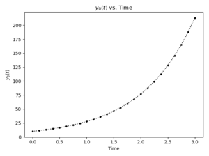
where \(C\) is again some constant. The following code will calculate the population for a span of 3 seconds with 25 points for the population model above with an initial population of 10 and a constant of proportionality of 1.02:

# %% Imports
import numpy as np
import matplotlib.pyplot as plt
from scipy.integrate import solve_ivp
from ode_helpers import state_plotter

# %% Define derivative function
def f(t, y, c):
    dydt = [c[0] * y[0]]
    return dydt
    
# %% Define time spans, initial values, and constants
tspan = np.linspace(0, 3, 25)
yinit = [10]
c = [1.02]

# %% Solve differential equation
sol = solve_ivp(lambda t, y: f(t, y, c), 
                [tspan[0], tspan[-1]], yinit, t_eval=tspan)

# %% Plot states
state_plotter(sol.t, sol.y, 1)

Multiple Variable Models

Result for system with two variables

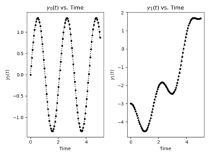
It is possible to solve multiple-variable systems by making sure the differential function returns values for each of the variables. For instance, in the following system the first variable's rate of change depends only on time while the second is dependent upon both time and the first variable:

\( \begin{align} \frac{dy_0}{dt}&=\alpha\cos(\beta t) & \frac{dy_1}{dt}&=\gamma y_0+\delta t \end{align} \)

The differential function f for this system will have a 2 element list as the output. Also, if you have systems with multiple dependent variables, just be sure to put the initial conditions in a list. For example, with the system defined as:

\( \begin{align} \frac{dy_0}{dt}&=4\cos(3t) & \frac{dy_1}{dt}&=-2y_1+0.5t \end{align} \)

you could use the following script to solve for both \(y_0\) and \(y_1\); the code assumes \(y_0\) starts as 0 and \(y_1\) starts at -3:

# %% Imports
import numpy as np
import matplotlib.pyplot as plt
from scipy.integrate import solve_ivp
from ode_helpers import state_plotter

# %% Define derivative function
def f(t, y, c):
    dydt = [c[0]*np.cos(c[1]*t), c[2]*y[0]+c[3]*t]
    return dydt

# %% Define time spans, initial values, and constants
tspan = np.linspace(0, 5, 100)
yinit = [0, -3]
c = [4, 3, -2, 0.5]

# %% Solve differential equation
sol = solve_ivp(lambda t, y: f(t, y, c), 
                [tspan[0], tspan[-1]], yinit, t_eval=tspan)

# %% Plot states
state_plotter(sol.t, sol.y, 1)

Higher Order Differential Equations

Result using constant third derivative.

The system must be written in terms of first-order differential equations only. To solve a system with higher-order derivatives, you will first write a cascading system of simple first-order equations then use them in your differential function. For example, assume you have a system characterized by constant jerk:

\( \begin{align} j&=\frac{d^3y}{dt^3}=C \end{align} \)

The first thing to do is write three first-order differential equations to represent the third-order equation:

\( \begin{align} y_0 &=y &~& &~\\ \frac{dy_0}{dt}&=\frac{dy}{dt}=y_1 & &\longrightarrow & \frac{dy_0}{dt}&=y_1\\ \frac{dy_1}{dt}&=\frac{d^2y_0}{dt^2}=\frac{d^2y}{dt^2}=y_2 & &\longrightarrow & \frac{dy_1}{dt}&=y_2\\ \frac{dy_2}{dt}&=\frac{d^2y_1}{dt^2}=\frac{d^3y_0}{dt^3}=\frac{d^3y}{dt^3}=j=C & &\longrightarrow & \frac{dy_2}{dt}&=C \end{align}\)

Notice how the derivatives cascade so that the constant jerk equation can now be written as a set of three first-order equations. Note that in this system, y[0] represents the position, y[1] represents the velocity, and y[2] represents the acceleration. This type of cascading system will show up often when modeling equations of motion.

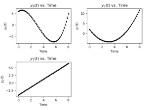
The following script, RunJerkDiff.m, calculates the position, velocity, and speed over a period of 8 seconds assuming an initial position of 6, and initial velocity of 2, an initial acceleration of -4, and a constant jerk of 1.3:

# %% Imports
import numpy as np
import matplotlib.pyplot as plt
from scipy.integrate import solve_ivp
from ode_helpers import state_plotter

# %% Define derivative function
def f(t, y, c):
    dydt = [y[1], y[2], c[0]]
    return dydt

# %% Define time spans, initial values, and constants
tspan = np.linspace(0, 8, 50)
yinit = [6, 2, -4]
c = [1.3]

# %% Solve differential equation
sol = solve_ivp(lambda t, y: f(t, y, c), 
                [tspan[0], tspan[-1]], yinit, t_eval=tspan)

# %% Plot states
state_plotter(sol.t, sol.y, 1)

Questions

Post your questions by editing the discussion page of this article. Edit the page, then scroll to the bottom and add a question by putting in the characters *{{Q}}, followed by your question and finally your signature (with four tildes, i.e. ~~~~). Using the {{Q}} will automatically put the page in the category of pages with questions - other editors hoping to help out can then go to that category page to see where the questions are. See the page for Template:Q for details and examples.