Python:Logical Masks

Introduction

Many times, you will see functions that are written in some kind of piecewise fashion. That is, depending upon that value of the input argument, the output argument may be calculated in one of several different ways. In these cases, you can use Python and NumPy's logical and relational arguments to create logical masks - arrays containing either 0's or 1's - to help determine the appropriate calculation to perform to determine the values in an array.

Important Notes

• All of the example codes assume you have already run (or have included in your script)

import math as m
import numpy as np
import matplotlib.pyplot as plt

Piecewise Constant

Sometimes, piecewise functions are broken up into several regions, with each region being defined by a single constant. These are called piecewise constant functions and can be easily generated in Python with NumPy.

Example - GPA Calculation

Take for example GPA as a function of numerical grade (assume \(\pm\)do not exist for the moment...). The mathematical statement of GPA might be:

\( \mbox{GPA}(\mbox{Grade})=\left\{ \begin{array}{rl} \mbox{Grade}\geq 90~~~ & 4\\ 80\leq\mbox{Grade} ~\And~ \mbox{Grade}<90~~~ & 3\\ 70\leq\mbox{Grade} ~\And~ \mbox{Grade}<80~~~ & 2\\ 60\leq\mbox{Grade} ~\And~ \mbox{Grade}<70~~~ & 1\\ \mbox{Grade}<60~~~ & 0 \end{array} \right. \)

If you want to write this table as a function that can accept multiple inputs at once, you really should not use an if-tree (because if-trees can only run one program segment for the entire matrix) or a for loop (because for loops are slower and more complex for this particular situation). Instead, use NumPy's ability to create logical masks. Look at the following code:

Grade=np.linspace(0, 100, 1000)
MaskForA = Grade>=90

The variable MaskForA will be the same size of the Grade variable, and will contain only True and False values. Given that, you can use this in conjunction with the function for an "A" grade to start building the GPA variable if you recall that True evaluates to 1 and False to 0:

Grade=np.linspace(0, 100, 1000)
MaskForA = Grade>=90
FunctionForA = 4
GPA = MaskForA*FunctionForA

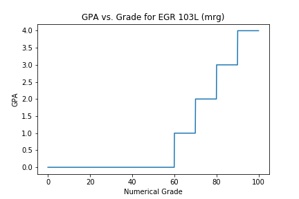
At the end of this script, the GPA variable will contain a 4 wherever the logical mask MaskForA was True and it will contain a 0 wherever the logical mask was False. All that is required is to extend this to the rest of the possible GPA's - the full code for a function is in the section below, along with an image of the graph it will create. Note the use of an outer set of parentheses to write the commands in the same visual way the function definition is written - this is not required, but does make the code easier to interpret.

Code and Graph

import numpy as np
import matplotlib.pyplot as plt


def num_to_gpa(grade):
    out = (
        (grade >= 90) * (4)
        + ((80 <= grade) & (grade < 90)) * (3)
        + ((70 <= grade) & (grade < 80)) * (2)
        + ((60 <= grade) & (grade < 70)) * (1)
        + (grade < 60) * (0)
    )
    return out


if __name__ == "__main__":

    grades = np.linspace(0, 100, 1000)
    GPA = num_to_gpa(grades)

    fig = plt.figure(num=1, clear=True)
    ax = fig.add_subplot(1, 1, 1)
    ax.plot(Grade, GPA)
    ax.set(
        xlabel="Numerical Grade", ylabel="GPA", 
        title="GPA vs. Grade for EGR 103L (mrg)"
    )
    fig.tight_layout()
    fig.savefig("GPAPlot.png")

For a further explanation, look at the following script. It investigates the individual masks for each grade for an array containing eight different grades:

ClassGrades = np.array([95, 70, 68, 38, 94, 84, 92, 87])
MaskForA = ClassGrades>=90
MaskForB = (80<=ClassGrades) & (ClassGrades<90)
MaskForC = (70<=ClassGrades) & (ClassGrades<80)
MaskForD = (60<=ClassGrades) & (ClassGrades<70)
MaskForF = ClassGrades<60

The masks now look like:

MaskForA: array([ True, False, False, False,  True, False,  True, False])
MaskForB: array([False, False, False, False, False,  True, False,  True])
MaskForC: array([False,  True, False, False, False, False, False, False])
MaskForD: array([False, False,  True, False, False, False, False, False])
MaskForF: array([False, False, False,  True, False, False, False, False])

and the products of each of the masks with each of the relevant GPA values would produce:

MaskForA*FunctionForA: array([4, 0, 0, 0, 4, 0, 4, 0])
MaskForB*FunctionForB: array([0, 0, 0, 0, 0, 3, 0, 3])
MaskForC*FunctionForC: array([0, 2, 0, 0, 0, 0, 0, 0])
MaskForD*FunctionForD: array([0, 0, 1, 0, 0, 0, 0, 0])
MaskForF*FunctionForF: array([0, 0, 0, 0, 0, 0, 0, 0])

These five matrices are added together to give:

GPA: array([4, 2, 1, 0, 4, 3, 4, 3])

Non-constant Piecewise Functions

Sometimes, piecewise functions are defined as following different formulas involving the independent variable over a range of inputs rather than being piece-wise constant.

Example 1 - Discrete Function

For example, the expression:

\( f(x)=\left\{ \begin{array}{rl} x<0 & 0\\ 0\leq x<5 & x\\ 5\leq x<10 & 5\\ x\geq 10 & 2x-15 \end{array} \right. \)

which, for integers -2 through 12 can be calculated and graphed:

Code and Graph

import numpy as np
import matplotlib.pyplot as plt

def fun(x):
    out = (
        (x<0) * (0) + 
        ((0<=x) & (x<5)) * (x) + 
        ((5<=x) & (x<10)) * (5) + 
        (x>=10) * (2*x-15))
    return out

if __name__ == "__main__":
    
    xvals = np.arange(-2, 13)
    yvals = fun(xvals)
    fig = plt.figure(num=1, clear=True)
    ax = fig.add_subplot(1, 1, 1)
    ax.stem(xvals, yvals)
    ax.set(xlabel='x', ylabel='f(x)',
           title ='Piecewise Function (NetID)')
    fig.tight_layout()
    fig.savefig('PFunction.png')

Intermediate Results

Several of the intermediate results are presented below. You will not have any of this in your programs. Also, note that the spacing in this document is set to make it easier to see which elements in one variable are paired up with equivalent elements in another variable (for example, to determine the element-multiplication of Mask 2 and Function 2). Note that the masks are shown below as arrays with 1 representing True and 0 representing False in order to save space:

(x>0) * 1:                  array([1, 1, 0, 0, 0, 0, 0, 0, 0, 0, 0, 0, 0, 0, 0])
((0<=x) & (x<5)) * (x) * 1: array([0, 0, 1, 1, 1, 1, 1, 0, 0, 0, 0, 0, 0, 0, 0])
((5<=x) & (x<10)) * 1:      array([0, 0, 0, 0, 0, 0, 0, 1, 1, 1, 1, 1, 0, 0, 0])
(x>=10) * 1:                array([0, 0, 0, 0, 0, 0, 0, 0, 0, 0, 0, 0, 1, 1, 1])

Notice how the masks end up spanning the entire domain of \(x\) without overlapping. The functions - as calculated over the entire domain, are:

Function 1: 0
Function 2: array([-2, -1,  0,  1,  2,  3,  4,  5,  6,  7,  8,  9, 10, 11, 12])
Function 3: 5
Function 4: array([-19, -17, -15, -13, -11,  -9,  -7,  -5,  -3,  -1,   1,   3,   5,  7,   9])

The individual products of the masks and the functions give:

Mask 1 *Function 1: array([0, 0, 0, 0, 0, 0, 0, 0, 0, 0, 0, 0, 0, 0, 0])
Mask 2 *Function 2: array([0, 0, 0, 1, 2, 3, 4, 0, 0, 0, 0, 0, 0, 0, 0])
Mask 3 *Function 3: array([0, 0, 0, 0, 0, 0, 0, 5, 5, 5, 5, 5, 0, 0, 0])
Mask 4 *Function 4: array([0, 0, 0, 0, 0, 0, 0, 0, 0, 0, 0, 0, 5, 7, 9])

Finally, when these are all added together, none of the individual products interfere with each other, so:

f: array([0, 0, 0, 1, 2, 3, 4, 5, 5, 5, 5, 5, 5, 7, 9])

Example 2 - Acceleration Due To Gravity

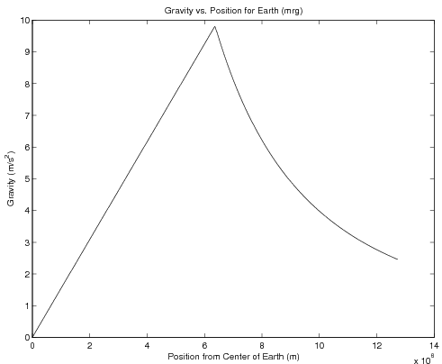
The following example determines the acceleration due to gravity for a sphere a particular distance away from the center of a sphere of constant density \(\rho\) and radius R. The formula changes depending on whether you are inside the sphere's surface or not. That is:

\( \mbox{Gravity}(r)= \left\{ \begin{array}{lr} r<=R & \frac{4}{3}\pi G\rho r\\ r>R & \frac{4}{3}\pi G \rho\frac{R^3}{r^2} \end{array} \right. \)

You can use the same method as the example above, making sure to calculate the values of the function rather than simply using constants. The following code and graph demonstrate:

Code and Graph

G = 6.67e-11
rho = 5515
R = 6371e3
Position = np.linspace(0.1, 2*R, 1000)
MaskForInside = Position<=R
FunctionForInside = 4/3*m.pi*G*rho*Position
MaskForOutside = Position>R
FunctionForOutside = 4/3*m.pi*G*rho*R**3/Position**2
Gravity = \
     MaskForInside*FunctionForInside + \
     MaskForOutside*FunctionForOutside
plt.plot(Position, Gravity, 'k-');
plt.xlabel('Position from Center of Earth ($m$)');
plt.ylabel('Gravity ($m/s^2$)');
plt.title('Gravity vs. Position for Earth (mrg)');
plt.savefig('GravityPlot.png')

Using Logical Masks in Functions

Any of these tasks can be done using functions. For example, you could use a function in the script to compute the gravity - in this case G could be defined in the function, the density and radius of the planet in question could be passed along (with Earth value as the default, because, astronomical narcissism), and the rest of the work could be in the script itself.

def grav_fun(r, rho=5515, R=6371e3):
    # Note: defaults to Earth
    G = 6.67e-11
    return (r<=R) * (4/3*m.pi*G*rho*r) + \
           (r>R)  * (4/3*m.pi*G*rho*R**3/r**2)

Position = np.linspace(0.1, 2*R, 1000)
plt.plot(Position, grav_fun(Position), 'k-')
plt.xlabel('Position from Center of Earth (m)')
plt.ylabel('Gravity (m/s^2)')
plt.title('Gravity vs. Position for Earth (mrg)')
plt.savefig('GravityPlot.png')

Questions

Post your questions by editing the discussion page of this article. Edit the page, then scroll to the bottom and add a question by putting in the characters *{{Q}}, followed by your question and finally your signature (with four tildes, i.e. ~~~~). Using the {{Q}} will automatically put the page in the category of pages with questions - other editors hoping to help out can then go to that category page to see where the questions are. See the page for Template:Q for details and examples.