Maple/Differential Equations/RC Example

Description

The following page will go through an example of using Maple's ability to work with differential equations to analyze a circuit that undergoes a change in source values. In this particular case, the independent source is given as a constant for all times before 0 sec, at which time it changes to a non-constant source. The source is connected to a network containing both resistors and a capacitor. While there are several ways to put all this work together in a Maple script, the following will provide a flexible framework for solving the equations and using substitution to determine a numerical list of initial conditions, substituting element values into the differential equations and putting them into a list, solving the differential equations, and finally plotting the results.

Circuit

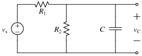
For this demonstration code, the following circuit is used:

where \(R_1\)=20 k\(\Omega\), \(R_2\)=30 k\(\Omega\), \(C\)=50 \(\mu\)F, and \(v_s(t)\) changes from 5 V to 10 cos(8\(t\)) V when \(t=0\) s.

DC Steady-State Analysis

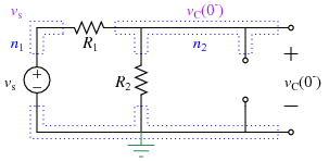
Assuming the circuit has been in place for a "long time" before \(t\)=0 sec, and given the topology of the circuit and the fact that the independent source is a constant for all times before 0 sec, you can use the DC steady-state equivalent for the circuit at \(t=0^-\) sec:

Using KCL at the top right node gives:

\( \frac{v_C(0^-)-v_s}{R_1}+ \frac{v_C(0^-)}{R_2}=0\! \)

which can be solved to find the capacitor voltage at the time just before the source \(v_s(t)\) changes.

Model Equations for t>0

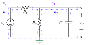
In general, after \(t\)=0 sec you can label the circuit as:

Using KCL at the top right node again gives:

\( \frac{v_C-v_s}{R_1}+ \frac{v_C}{R_2}+C\frac{dv_C}{dt}=0\! \)

Code

Now that the equations for DC steady state and for the differential model are known, you can write Maple code to solve for everything.

Preparing the Worksheet

Be sure that your name and the assignment show up as text at the top of the page. Also be sure that the first Maple command is restart.

Element and Source Values

Next, generate lists for the element values and for the source values. For the element values, you can write

ElementVals:= R1=20e3, R2=30e3, C=50e-6

For the source values, there will be two different sets - one before the transition and one after. The initial conditions will be based on the old set while the differential equations will be based on the new. For that reason, there need to be two different lists:

OldSourceVals:= vs(t)=5
NewSourceVals:= vs(t)=10*cos(8*t)

Note that the lists have the source values as functions of t - this will come in handy in solving circuits with time-varying inputs.

Initial Conditions From Steady-State

While Maple can solve differential equations with symbolic initial conditions and coefficients, most of the time this will result in a very unwieldy and unhelpful representation. For this assignment, you will be providing Maple with numerical values for the initial conditions. The three step process for this is to set up equations for the DC steady-state values in terms of the sources and elements:

ss1 := (vcss-vs(t))/R1 + vcss/R2 = 0

solve those equations,

ICsoln := solve({ss1}, [vcss])

and then substitute in the proper element and source values.

ICnum := subs(ICsoln[], ElementVals, OldSourceVals, {vc(0) = vcss})

This latter part will also be where you explicitly tell Maple that the steady state values are the initial conditions by stating that vc(0) is equal to the numerical value of vcss. The output of this should be a set of equations, where sets are surrounded by curly brackets.

Differential Equations

Next set up the differential equations, generate a single list of the differential equations with numerical values substituted in for the elements and sources, and solve. This is a three step process: define the equations:

eqn1 := (vc(t)-vs(t))/R1+vc(t)/R2+C*(diff(vc(t), t)) = 0

and then substitute in the element values and the new source values:

EQnum := subs(ElementVals, NewSourceVals, {eqn1})

The end result will be a set of equations. Now solve the equations:

MySoln := dsolve({EQnum[], ICnum[]}, [vc(t)])

You may want to look at a simplified version of the solution:

simplify(evalf[4](MySoln))

Note that in many cases the results of the differential equation are, frankly, ugly. Sometimes, telling Maple to solve using the Laplace method comes up with a more compact answer:

MySoln := dsolve({EQnum[], ICnum[]}, [vc(t)], method=laplace):
simplify(evalf[4](MySoln))

Other times, neither Maple's default method nor Laplace have a ``nice answer; in those cases, simply put a colon at the end of the line to suppress the output and forget about the simplify line:

MySoln := dsolve({EQnum[], ICnum[]}, [vc(t)]):

In those cases, you will want to focus more on the plot than the analytical solution.

Plotting

Plotting can sometimes be a little more complicated than it seems - much of the time, round-off errors will cause solutions that have tiny vestigial imaginary values. To eliminate this, you can have Maple map the real part of the solution vector. That is:

plot(map(Re, subs(MySoln, [vc(t)])), t = 0 .. 5, 
labels = ["Time (t)", "Voltage (V)"], 
labeldirections = [horizontal, vertical], 
title = "Capacitor Voltage", legend = ["vc"]);

Complete Example

For the Spring 2015 semester, students in EGR 224 can copy the code from:

/afs/acpub.duke.edu/courses/2015_spr/egr/224l/public/lab3/DemonstrationCode.mw

Here is the complete, paste-able worksheet, but see the note below before copying and pasting.

# Demonstration Code - RC Circuit

# Prepare Worksheet
restart;

# Element and Source Values
ElementVals := R1 = 20e3, R2 = 30e3, C = 50e-6;
OldSourceVals := vs(t) = 5;
NewSourceVals := vs(t) = 10*cos(8*t);

# Initial Conditions
ss1 := (vcss-vs(t))/R1+vcss/R2 = 0;
ICsoln := solve({ss1}, [vcss]);
ICnum := subs(ICsoln[], ElementVals, OldSourceVals, {vc(0) = vcss});

# Differential Equations
eqn1 := (vc(t)-vs(t))/R1+vc(t)/R2+C*(diff(vc(t), t)) = 0;
EQnum := subs(ElementVals, NewSourceVals, {eqn1});
MySoln := dsolve({EQnum[], ICnum[]}, [vc(t)], method = laplace);
simplify(evalf[4](MySoln));

#Plotting
plot(subs(MySoln, map(Re, [vc(t)])), t = 0 .. 5, labels = ["Time (t)", "Voltage (V)"], labeldirections = [horizontal, vertical], title = "Capacitor Voltage", legend = ["vc"]);

Note - you may want to copy each line into its own execution group. There does not seem to be a simple way to cope and paste a file like this and have each command land in its own execution group. If anyone figures out a good way to solve this problem, please add it here.