Difference between revisions of "Simulink/Tutorials/Signals"
m |
|||
| (20 intermediate revisions by the same user not shown) | |||
| Line 1: | Line 1: | ||
| + | <!-- EGR 224 specific | ||
This lab focuses on introducing MATLAB and Simulink and using | This lab focuses on introducing MATLAB and Simulink and using | ||
them to analyze transfer functions and numerically solve | them to analyze transfer functions and numerically solve | ||
differential equations. | differential equations. | ||
Many engineering problems can be easily modeled using block | Many engineering problems can be easily modeled using block | ||
| − | diagrams. | + | diagrams. |
| − | |||
In the Alciatore and Histand book, block diagrams are used | In the Alciatore and Histand book, block diagrams are used | ||
as early as Figure 1.3 to graphically illustrate the connection of | as early as Figure 1.3 to graphically illustrate the connection of | ||
| Line 13: | Line 13: | ||
--> | --> | ||
| − | The creators of MATLAB understand that block diagrams are used to | + | The creators of [[MATLAB]] understand that block diagrams are used to |
visually depict complicated systems, and also that | visually depict complicated systems, and also that | ||
the mathematical characteristics of those systems, once defined, can | the mathematical characteristics of those systems, once defined, can | ||
be used to determine the values for the various signals throughout the | be used to determine the values for the various signals throughout the | ||
| − | system. For that reason, they developed the Simulink package as an | + | system. For that reason, they developed the [[Simulink]] package as an |
add-on to MATLAB. Simulink allows you to draw your system as if you | add-on to MATLAB. Simulink allows you to draw your system as if you | ||
were drawing a block diagram, and then to simulate the system using a | were drawing a block diagram, and then to simulate the system using a | ||
| Line 29: | Line 29: | ||
introduction, you should be able to generate a wide variety of | introduction, you should be able to generate a wide variety of | ||
signals, perform basic and intermediate mathematical operations, | signals, perform basic and intermediate mathematical operations, | ||
| − | visualize and save data, control models with a script, and print your model. | + | visualize and save data, control models with a script (not completed yet), and print your model. |
| + | |||
| + | Note - figures are numbered by section. I haven't figured out a better way to do this... | ||
==Starting Simulink== | ==Starting Simulink== | ||
| Line 47: | Line 49: | ||
[[Image:SDDemoSigGen.png|thumb|Figure 1]] | [[Image:SDDemoSigGen.png|thumb|Figure 1]] | ||
The Simulink library is broken up into several categories, and each category contains several building blocks for modeling signals and systems. To look at the contents of a particular category, just double-click its name in the library window. For example, if you double-click on the <code>Sources</code> icon, you will open a new library window containing several different ways that MATLAB can generate a signal. If you want to add one of these to your model, all you have to do is click and hold on it with the left mouse button, then drag it onto your canvas. Try this with the <code>Signal Generator</code> block. Your model should now have a single <code>Signal Generator</code> (fig. 1). | The Simulink library is broken up into several categories, and each category contains several building blocks for modeling signals and systems. To look at the contents of a particular category, just double-click its name in the library window. For example, if you double-click on the <code>Sources</code> icon, you will open a new library window containing several different ways that MATLAB can generate a signal. If you want to add one of these to your model, all you have to do is click and hold on it with the left mouse button, then drag it onto your canvas. Try this with the <code>Signal Generator</code> block. Your model should now have a single <code>Signal Generator</code> (fig. 1). | ||
| − | |||
To examine and change the possible parameters of a block, simply | To examine and change the possible parameters of a block, simply | ||
| Line 55: | Line 56: | ||
amplitude of the signal, the frequency, and what units of | amplitude of the signal, the frequency, and what units of | ||
frequency to use. If | frequency to use. If | ||
| − | you were to want to use an input of <math>x(t)=\sin(8t)</math>, for example, you would | + | you were to want to use an input of <math>x(t)=3\sin(8t)</math>, for example, you would |
| − | choose a sine wave, using the simulation time, with an amplitude of | + | choose a sine wave, using the simulation time, with an amplitude of 3 |
and a frequency of 8 radians per second. Go ahead and make those | and a frequency of 8 radians per second. Go ahead and make those | ||
changes, then click the <code>OK</code> button to accept them. | changes, then click the <code>OK</code> button to accept them. | ||
| + | <br clear=all> | ||
| + | |||
[[Image:SDDemoGain.png|thumb|Figure 2]] | [[Image:SDDemoGain.png|thumb|Figure 2]] | ||
| Line 70: | Line 73: | ||
now you have a Signal Generator and a Gain block. Move the Gain block | now you have a Signal Generator and a Gain block. Move the Gain block | ||
so it is about an inch to the right of the Signal Generator (fig. 2). | so it is about an inch to the right of the Signal Generator (fig. 2). | ||
| + | <br clear=all> | ||
[[Image:SDDemoGain2.png|thumb|Figure 3]] | [[Image:SDDemoGain2.png|thumb|Figure 3]] | ||
| Line 78: | Line 82: | ||
<code>Apply</code> button. Notice that the number inside the block itself | <code>Apply</code> button. Notice that the number inside the block itself | ||
changes as a result (fig. 3). | changes as a result (fig. 3). | ||
| + | <br clear=all> | ||
[[Image:SDDemoGainK.png|thumb|Figure 4]] | [[Image:SDDemoGainK.png|thumb|Figure 4]] | ||
| Line 93: | Line 98: | ||
different inputs. In this case, change the gain back to 2 and hit | different inputs. In this case, change the gain back to 2 and hit | ||
<code>OK</code>, then make the gain block a more normal size. | <code>OK</code>, then make the gain block a more normal size. | ||
| + | <br clear=all> | ||
[[Image:SDDemoOuts.png|thumb|Figure 6]] | [[Image:SDDemoOuts.png|thumb|Figure 6]] | ||
| Line 103: | Line 109: | ||
the <code>Gain</code> block, with the <code>Scope</code> about an inch above and the | the <code>Gain</code> block, with the <code>Scope</code> about an inch above and the | ||
<code>To Workspace</code> about an inch below (fig. 6). | <code>To Workspace</code> about an inch below (fig. 6). | ||
| + | <br clear=all> | ||
If you double-click the scope, an oscilloscope window will appear. | If you double-click the scope, an oscilloscope window will appear. | ||
| Line 120: | Line 127: | ||
notice that the name of the variable is now showing inside of the | notice that the name of the variable is now showing inside of the | ||
block (fig. 7). | block (fig. 7). | ||
| + | <br clear=all> | ||
[[Image:SDDemoWire1.png|thumb|Figure 8]] | [[Image:SDDemoWire1.png|thumb|Figure 8]] | ||
| Line 133: | Line 141: | ||
cursor changes to double crosshairs when you have found a terminus for | cursor changes to double crosshairs when you have found a terminus for | ||
your wire. Now connect the output of the <code>Gain</code> block to the <code>Scope</code> (fig. 8). | your wire. Now connect the output of the <code>Gain</code> block to the <code>Scope</code> (fig. 8). | ||
| + | <br clear=all> | ||
If you also want to connect the <code>Gain</code> block to the | If you also want to connect the <code>Gain</code> block to the | ||
| Line 160: | Line 169: | ||
==Running Simulations== | ==Running Simulations== | ||
| − | [[Image:SDDemoPlotVS.png|thumb|Plot with no limit on maximum step size]] | + | [[Image:SDDemoPlotVS.png|thumb|Fig 1: Plot with no limit on maximum step size]] |
| − | [[Image:SDDemoPlotVS2.png|thumb|Plot with limit of 0.01 on maximum step size]] | + | [[Image:SDDemoPlotVS2.png|thumb|Fig 2: Plot with limit of 0.01 on maximum step size]] |
Now that you have a basic block diagram with an input signal going | Now that you have a basic block diagram with an input signal going | ||
| Line 193: | Line 202: | ||
</source> | </source> | ||
in MATLAB's command window | in MATLAB's command window | ||
| − | to plot the signal - you should get fig | + | to plot the signal - you should get fig. 1. |
When you do this, you will notice something very | When you do this, you will notice something very | ||
| Line 208: | Line 217: | ||
<code>Max step size</code> to a reasonable value | <code>Max step size</code> to a reasonable value | ||
for the speed of the signal - perhaps 0.01. Re-run the simulation, | for the speed of the signal - perhaps 0.01. Re-run the simulation, | ||
| − | and re-plot your results to get fig | + | and re-plot your results to get fig. 2. |
<br clear=all> | <br clear=all> | ||
==Creating Arbitrary Inputs== | ==Creating Arbitrary Inputs== | ||
| − | [[Image:SDDemo2uc.png|thumb| | + | [[Image:SDDemo2uc.png|thumb|Fig. 1: After deleting blocks]] |
| − | [[Image:SDDemo2c.png|thumb| | + | [[Image:SDDemo2c.png|thumb|Fig. 2: After adding new blocks]] |
| − | [[Image:SDDemo2cPlot.png|thumb| | + | [[Image:SDDemo2cPlot.png|thumb|Fig. 3: Plot of new output]] |
There are several ways to create different inputs signals. The Signal | There are several ways to create different inputs signals. The Signal | ||
| Line 228: | Line 237: | ||
Now select and delete both the <code>Signal Generator</code> and the | Now select and delete both the <code>Signal Generator</code> and the | ||
<code>Gain</code> block. Among other changes, you will now be left with | <code>Gain</code> block. Among other changes, you will now be left with | ||
| − | unconnected lines, denoted by red dotted lines (fig | + | unconnected lines, denoted by red dotted lines (fig 1). |
These can be deleted by selecting them and hitting delete, or they | These can be deleted by selecting them and hitting delete, or they | ||
can be reused by putting a block's input or output ports close enough | can be reused by putting a block's input or output ports close enough | ||
| Line 243: | Line 252: | ||
can drag the <code>Fcn</code> block again or use the arrow keys to move | can drag the <code>Fcn</code> block again or use the arrow keys to move | ||
it until it connects and the wire turns solid black. You should now | it until it connects and the wire turns solid black. You should now | ||
| − | have the model in fig | + | have the model in fig 2. |
To enter a function, double-click the <code>Fcn</code> block. Note that the | To enter a function, double-click the <code>Fcn</code> block. Note that the | ||
| Line 257: | Line 266: | ||
Once you have that function entered, re-run the simulation. If you | Once you have that function entered, re-run the simulation. If you | ||
make a plot of <code>y</code> as a function of <code>tout</code> using the command | make a plot of <code>y</code> as a function of <code>tout</code> using the command | ||
| − | <code>plot(tout, y)</code>, you should get the plot in fig | + | <code>plot(tout, y)</code>, you should get the plot in fig. 3. |
| + | |||
| + | <br clear=all> | ||
==Transferring Data== | ==Transferring Data== | ||
| Line 272: | Line 283: | ||
name you want to change. This can be very useful if your blocks have | name you want to change. This can be very useful if your blocks have | ||
real-world analogs. You can also probably come up with much more | real-world analogs. You can also probably come up with much more | ||
| − | interesting names than | + | interesting names than <code>To Workspace</code> for your outputs. Avoid using |
dots or slashes in the block names, however. Stick with letters and | dots or slashes in the block names, however. Stick with letters and | ||
numbers if at all possible. This will become more important in the | numbers if at all possible. This will become more important in the | ||
| Line 286: | Line 297: | ||
==Running Models With Scripts== | ==Running Models With Scripts== | ||
| + | This section is under construction and not required for EGR 224 Spring 2010 | ||
| + | <!-- | ||
Another way to run a model, besides using the <code>Simulation</code> menu, | Another way to run a model, besides using the <code>Simulation</code> menu, | ||
is to write a script that interacts with the model. The advantages of | is to write a script that interacts with the model. The advantages of | ||
| Line 400: | Line 413: | ||
passed through it, and type <code>help sim</code> for more information about | passed through it, and type <code>help sim</code> for more information about | ||
the <code>sim</code> command. | the <code>sim</code> command. | ||
| + | --> | ||
==Saving and Printing Models== | ==Saving and Printing Models== | ||
| Line 409: | Line 423: | ||
</source> | </source> | ||
The following code will not only print the model based on the | The following code will not only print the model based on the | ||
| − | filename, it will also save and close the model window when the script | + | filename, it will also save and close the model window when |
| − | + | <!-- the script is--> | |
| + | finished: | ||
<source lang="matlab"> | <source lang="matlab"> | ||
| + | Filename = 'StringGoesHere' | ||
eval(sprintf('print -s%s -deps %smodel', Filename, Filename)) | eval(sprintf('print -s%s -deps %smodel', Filename, Filename)) | ||
save_system(Filename) | save_system(Filename) | ||
| Line 428: | Line 444: | ||
==Sample Codes and Models== | ==Sample Codes and Models== | ||
| + | <!-- | ||
\subsection{RunLab2WithScript.m\label{Sim:Runner}} | \subsection{RunLab2WithScript.m\label{Sim:Runner}} | ||
\listinginput[1]{1}{./SIMULINK/RunLab2Demo2c.m} | \listinginput[1]{1}{./SIMULINK/RunLab2Demo2c.m} | ||
| Line 435: | Line 452: | ||
\epsfig{file=./SIMULINK/Lab2WithScriptmodel.eps} | \epsfig{file=./SIMULINK/Lab2WithScriptmodel.eps} | ||
\end{center} | \end{center} | ||
| + | --> | ||
| − | + | {{Protected Class Document}} | |
| − | + | [[Category: EGR 224]] | |
| − | + | [[Category: ECE 382]] | |
| − | + | [[Category:ME 344]] | |
| − | |||
| − | |||
| − | |||
| − | |||
| − | |||
| − | |||
| − | |||
| − | |||
| − | |||
| − | |||
| − | |||
| − | |||
| − | |||
| − | |||
| − | |||
| − | |||
| − | |||
| − | |||
| − | |||
Latest revision as of 16:32, 19 February 2013
The creators of MATLAB understand that block diagrams are used to
visually depict complicated systems, and also that
the mathematical characteristics of those systems, once defined, can
be used to determine the values for the various signals throughout the
system. For that reason, they developed the Simulink package as an
add-on to MATLAB. Simulink allows you to draw your system as if you
were drawing a block diagram, and then to simulate the system using a
variety of computational methods, usually with some component of
integration involved.
This introduction will cover starting Simulink, understanding the basic blocks and connections, and running simulations. It will then move on to creating arbitrary functions, transferring data between the model and the workspace, and printing models. By the end of this introduction, you should be able to generate a wide variety of signals, perform basic and intermediate mathematical operations, visualize and save data, control models with a script (not completed yet), and print your model.
Note - figures are numbered by section. I haven't figured out a better way to do this...
Contents
Starting Simulink
Simulink is an add-on package to MATLAB, and OIT has purchased several
licenses for use on the Linux workstations. To start Simulink, you
must first start MATLAB (by typing matlab &), then type simulink
at the command prompt within MATLAB. At that point, the Simulink library window will come up.
While you will not be creating your model in this window, you will be
using it to obtain access to the many different built-in blocks that
Simulink provides.
To start your own model, go to File->New->Model. Now you have a blank canvas to work with. To fill it in, you need to
know what the basic blocks are, how to bring them into your model, and
how to connect them.
Basic Blocks and Connections
The Simulink library is broken up into several categories, and each category contains several building blocks for modeling signals and systems. To look at the contents of a particular category, just double-click its name in the library window. For example, if you double-click on the Sources icon, you will open a new library window containing several different ways that MATLAB can generate a signal. If you want to add one of these to your model, all you have to do is click and hold on it with the left mouse button, then drag it onto your canvas. Try this with the Signal Generator block. Your model should now have a single Signal Generator (fig. 1).
To examine and change the possible parameters of a block, simply
double-click on it in your model window.
The Signal Generator, for example, allows
you to choose what wave form you would like, the time base to use, the
amplitude of the signal, the frequency, and what units of
frequency to use. If
you were to want to use an input of \(x(t)=3\sin(8t)\), for example, you would
choose a sine wave, using the simulation time, with an amplitude of 3
and a frequency of 8 radians per second. Go ahead and make those
changes, then click the OK button to accept them.
Once you have some kind of input signal, you may want to process it.
There are many different ways to process a signal in Simulink, ranging
from basic mathematics to advanced image processing and frequency
analysis. For now, open up the Math Operations category by
double-clicking it in the original library window. Among the
different operations you can perform is the Gain block, which
acts like a multiplier. Drag a copy of this into your model, so that
now you have a Signal Generator and a Gain block. Move the Gain block
so it is about an inch to the right of the Signal Generator (fig. 2).
If you double-click
this block, you will see that it has more options than you may have
thought for a simple gain. Generally, however, you will only need to
change the Gain itself. Go ahead and set the gain to 2 and click the
Apply button. Notice that the number inside the block itself
changes as a result (fig. 3).
The number in the gain block will reflect the
actual gain if there is room for it - otherwise the gain block will
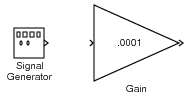
have the letter K in it. For example, if you put in 0.0001 for
the gain and hit Apply again, the block will just have a K in it (fig. 4).
If you really want to see the gain, you can change the size of
the block to make it large enough that the number will fit inside (fig. 5)
though generally you will not want to resize blocks just to see the
contents. The main blocks you will be resizing are those with
multiple inputs or outputs, for example, summation blocks there the
larger size will make it easier to track and attach the
different inputs. In this case, change the gain back to 2 and hit
OK, then make the gain block a more normal size.
Finally, you will want to have some way of viewing or saving the
data. If you go back to the original Library window and open up the
Sinks category, you will see the various ways that MATLAB can
take a signal and either send the information to the screen, to the
workspace, or to a file. In this case, you are going to want to both
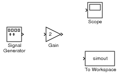
view and manipulate the data, so drag both a Scope and a To Workspace to your model. Put both about an inch to the right of
the Gain block, with the Scope about an inch above and the
To Workspace about an inch below (fig. 6).
If you double-click the scope, an oscilloscope window will appear.
The scope is useful for viewing the signals throughout a simulation in
real time. Generally, you will add these during the construction of a
model, but once you have completed the model, you will want a more
permanent record of the data obtained. This is where the To Workspace block comes in.
The To Workspace block will record the signal values sent to
it as a variable in
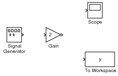
the MATLAB workspace. If you double-click on the block, you will note
that you can change the variable name - go ahead and make this y. The Save format that is most readily used is Array,
so go ahead
and make that change as well. The default cases for the other
parameters will generally work fine. Once done, click OK and
notice that the name of the variable is now showing inside of the
block (fig. 7).
Now that the blocks are in place, you need to connect them. You will
notice if you run the cursor over the small port symbol (the \(>\)) of a
block that the cursor changes from an arrow to crosshairs. The way
you connect blocks is to pick the port of one block, hold down the
left mouse button, and drag until you hit another port (or another
wire). Go ahead and connect the Signal Generator to the Gain block by
putting the cursor on top of the output port of the Signal Generator,
holding down the left mouse button, and dragging until the cursor is
over the input port of the Gain block. You will notice that the
cursor changes to double crosshairs when you have found a terminus for
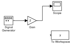
your wire. Now connect the output of the Gain block to the Scope (fig. 8).
If you also want to connect the Gain block to the
To Workspace block,
you will need to first click on the input of the To Workspace
then drag until you hit the wire connecting the scope to the
gain block. You cannot go back to the Gain block's output port,
because every input or output port can only be used once.
Since every wire should have at least one new port connection, you must begin from that port. Again, you will get the double crosshairs when you are over a wire such that a connection will be made and you will notice a node symbol (small black dot) at the connection. If you make a mistake and drop the wire before it is connected, you will get a dashed red wire with a port symbol at the end of it. You can remove this wire by left clicking on it (thereby selecting it) and hitting delete.
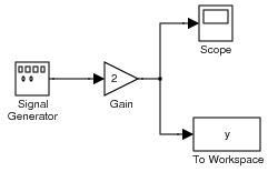
At this point, your model should have all four blocks properly wired,
with a gain of 2 and a To Workspace variable called \(y\) (fig. 9).
There should also be an open Scope window that came about when your
double-clicked the Scope block.
Running Simulations
Now that you have a basic block diagram with an input signal going
through a system that multiplies that signal by 2 as well as two
different ways of examining the data, you are ready to simulate the
system. Within the Simulation menu of your model,
go to Configuration Parameters and you will discover that Simulink has an extensive
array of options from which to choose. For now, the critical part is
telling MATLAB to store all the data and telling MATLAB the
simulation time.
Go to the Data Import/Export selection and un-check the
Limit data points... option in the Save options. For
whatever reason, MATLAB defaults on only storing the last thousand
data points unless you specify otherwise. Generally, you will want
Simulink to report all the data.
With respect to timing, go to the Solver selection.
The default case - which goes from 0 to
10 seconds - might work, so go ahead and hit OK.
Then, to run the simulation, go to Simulation and Start.
The scope will show the values of the output, and when the simulation
is finished, MATLAB will beep.
If you type whos in MATLAB, you will discover that not only did
you generate an array called y but that Simulink also created an
array called tout for you.
Now you can run the simulation and, when finished, issue the command
plot(tout, y)
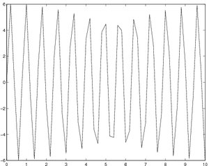
in MATLAB's command window to plot the signal - you should get fig. 1.
When you do this, you will notice something very
disturbing - the output signal does not look like a sine wave a 8
radians per second. This is because Simulink, while processing your
model, tries to solve as quickly as possible by taking as large a time
step as possible. For this particular model, allowing it to do that
has produces a somewhat disastrous result - the locations at which data
points were taken, if connected using lines, do not accurately
represent the signal.
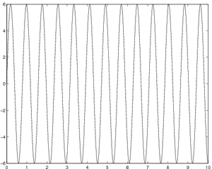
To forestall this, you can go
back into the Simulation menu's Configuration Parameters and make some
changes. Specifically, within the Solver selection change the
Max step size to a reasonable value
for the speed of the signal - perhaps 0.01. Re-run the simulation,
and re-plot your results to get fig. 2.
Creating Arbitrary Inputs
There are several ways to create different inputs signals. The Signal
Generator is certainly the easiest way to create a basic sinusoid,
square wave, or sawtooth. For other signals, you can use a
combination of sources and basic math to get what you want. There is
even a Signal Builder block that can be used to draw signals.
Generally, however, the easiest way to create an input is to use a
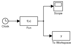
Clock block and feed it into a Fcn block. Go ahead and
save your current model as SDDemo1.mdl, then do a save as
and call it SDDemo2.mdl.
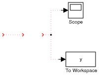
Now select and delete both the Signal Generator and the
Gain block. Among other changes, you will now be left with
unconnected lines, denoted by red dotted lines (fig 1).
These can be deleted by selecting them and hitting delete, or they
can be reused by putting a block's input or output ports close enough
that Simulink thinks they should be connected. For example, drag a
Clock block from the Sources category such that the output of
the Clock is near the left-most part of the left line. It will
attach itself to that wire, though the wire will remain red since its
output end is still unconnected.
Now open the User-Defined Functions category and drag a
Fcn block into your model, placing it in the space vacated by the
gain block. The Fcn block is larger that the Gain block
so you can only snag one of the wires. To get the other one, you
can drag the Fcn block again or use the arrow keys to move
it until it connects and the wire turns solid black. You should now
have the model in fig 2.
To enter a function, double-click the Fcn block. Note that the
expression is currently a function of the vector u. This vector
represents the different inputs to the block. Right now, we are only
using a single input - though later you can use multiplexers to send
multiple streams along a single line. Your function, therefore,
should be written in terms of u[1]. For example, if you want
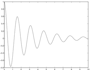
the output of the function to be \(e^{-t/3}\cos(4t)\), then the input to
this block should be exp(-u[1]/3)*cos(4*u[1]). Note - Simulink
does not like using the .* version of multiplication.
Once you have that function entered, re-run the simulation. If you
make a plot of y as a function of tout using the command
plot(tout, y), you should get the plot in fig. 3.
Transferring Data
As mentioned earlier, you will often want to transfer data from the
Simulink simulation to the workspace. The To Workspace block is
the easiest way to get a signal's information to the workspace. Just
make sure that the variable name is unique for each of the blocks and
that you have used the Array method for storing the data.
There are also From Workspace blocks if you want to pass in
value and time data from the workspace.
Naming and Arranging Blocks
You can change the name of blocks in Simulink by double-clicking the
name you want to change. This can be very useful if your blocks have
real-world analogs. You can also probably come up with much more
interesting names than To Workspace for your outputs. Avoid using
dots or slashes in the block names, however. Stick with letters and
numbers if at all possible. This will become more important in the
next section.
You may also occasionally want to aim a block in a different
direction - to do this, simply pick the block, then go to the
Format menu and select either Flip Block or Rotate
Block. You have already seen that you can resize blocks. Take note the
other options in the Format menu - there may be times with
particularly sophisticated models that you will want to use various
colors and other options to help clarify your system.
Running Models With Scripts
This section is under construction and not required for EGR 224 Spring 2010
Saving and Printing Models
To save a Simulink model, just go to the File menu and select either
Save or Save As. Simulink models should end with .mdl. To print your model, you can either use the Print function
in the File menu or type
print -deps -sMODELNAME FILENAME.eps
The following code will not only print the model based on the filename, it will also save and close the model window when finished:
Filename = 'StringGoesHere'
eval(sprintf('print -s%s -deps %smodel', Filename, Filename))
save_system(Filename)
close_system(Filename)
The name of the saved picture of the model will be
Filenamemodel.eps. If you are going to do several things
with the same model, you may
want to add some kind of flag in the sprintf command to
differentiate among plots. For example, if you are running code in a
loop based on some integer counter k, you could use the
following code:
eval(sprintf('print -s%s -deps %smodel_%0.0f', Filename, Filename, k))


