Symbolic/Examples/Circuits

Counting Equations

For an electric circuit containing only wires, sources, and resistances, three primary kinds of equations will help solve for the individual voltages and currents that may exist in the circuit. These are element equations, Kirchhoff's Current Law (KCL), and Kirchhoff's Voltage Law (KVL).

With respect to element equations, these can take multiple forms. For independent sources, the element equation is generally a value assigned to the source. For example, if there is a 10 V voltage source in the circuit, the element equation would be that the voltage across that element is 10 V. For resistances, the element equation is generally Ohm's Law

\( \begin{align*} v=iR \end{align*} \)

so long as the voltage and current are labeled using the passive sign convention. Finally, for dependent sources, the element equation will relate a voltage or current in the circuit to the dependent variable of the source. There will be as many element equations as there are elements, though typically independent source values are counted as "knowns" rather than "element equations."

For Kirchhoff's Current Law, the number of independent equations that can be generated by applying it will be one fewer than the number of nodes in the circuit. Note that this does not explicitly mean that KCL must only be applied at simple nodes - "supernodes" which combine multiple nodes may also be used, though care must be taken to make sure the combination of equations constitutes an independent set. Furthermore, there will be times when you might split a node into parts to determine currents flowing through specific wires that make up the node. For the brute force method, we will use simple nodes.

For Kirchhoff's Voltage Law, the number of independent equations that can be derived in a circuit consisting solely of two-terminal elements will be equal to:

\( \begin{align*} \mbox{KVL equations}=\mbox{elements}-\mbox{nodes}+1 \end{align*} \)

For planar circuits, this will be equal to the number of meshes in the circuit. There may be times when it is more efficient to use some superloop equations versus mesh equations, but for the brute force method with a planar circuit, we will use mesh equations.

Brute Force

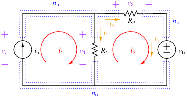
The following example shows the "brute force" method of setting up and solving for all the element currents and voltages for a simple resistive circuit and then using those solutions to solve for auxiliary information (in this case, some powers). The circuit involved is:

Equations

Element Equations

Mainly, these are Ohm's Law equations for the resistors, so:

\( \begin{align} R_1:& & v_1&=i_1R_1\\ R_2:& & v_2&=i_2R_2 \end{align} \)

KCL Equations

The number of independent KCL equations s one less than the number of nodes, so in this case, 2. Note: all three nodal KCL equations are written below, but node \(n_c\)'s is not used in the Maple worksheet.

\( \begin{align} KCL,n_a:& & -i_a+i_1+i_2&=0\\ KCL,n_b:& & -i_2+i_b&=0\\ KCL,n_c:& & i_a-i_1-i_b&=0 \end{align} \)

KVL Equations

The number of independent KVL equations is equal to the number of meshes for a 2-D circuit, or to the number of elements, minus the number of nodes, plus one for circuits in general. In this case, that is 2 independent KVL (two meshes, or 3 elements - 3 nodes + 1 = 2). For the brute force method, just use the mesh equations:

\( \begin{align} KVL,l_1:& & -v_a+v_1&=0\\ KVL,l_2:& & -v_1+v_2+v_b&=0 \end{align} \)

Auxiliary Equations

For this example, the auxiliary equations will be used to determine the power delivered by each source and the power absorbed by each resistor:

\( \begin{align} p_{del,i_a}&=v_ai_a & p_{del,v_b}&=-v_bi_b \\ p_{abs,R_1}&=v_1i_1 & p_{abs,R_2}&=v_2i_2 \end{align} \)

Note that all elements except for \(i_a\) are labeled passively.

Code

Maple

The Maple worksheet for this example is available in the Maple Cloud at this Maple Cloud Link. You can view the worksheet even if you do not have Maple; if you have Maple, you can download the worksheet and edit it.

The code assumes that:

\( \begin{align} R_1&=1000~\Omega & R_2&=2200~\Omega\\ i_a&=0.005~\mbox{A} & v_b&=12~\mbox{V} \end{align} \)

Python

Starting in 2022, we are looking at using Python to perform symbolic calculations. You can view three Notebook forms on a Google Drive Folder that has three versions of the example:

• "nosub" uses no subscripts for the variables; SymPy will automatically make variables with single digits at the end print with subscripts (like $$i_1$$) but will not do subscripts for things like $$ia$$
• "allsub" uses subscripts for all the variables - which requires also putting the subscripts in the code
• "dispsub" uses a two-step process for relating simple variable names like $$ia$$ to more complicated display forms such as $$i_a$$. It even relates the variable name $$pdelia$$ to the display form $$p_{del,{i_a}}$$

The notebooks pull the sym_helper file from its home on GitHub if needed.

You can look at the Trinket below, which will also grab sym_helper if needed. It uses the "nosub" version of the code because Trinket apparently, among other things, doesn't know how to make a subscript b print correctly...