Difference between revisions of "MATLAB:Fminbnd and fminsearch"
| (19 intermediate revisions by 3 users not shown) | |||
| Line 1: | Line 1: | ||
| − | + | == Introduction == | |
| + | This page discusses two different ways of getting MATLAB to find the minimum of a function (versus a data set) - '''fminbnd''' and '''fminsearch'''. The fminbnd command can find a ''single'' independent value that will minimize a one-dimensional function over a specific domain. The fminsearch command can find a single '''vector''' of values that will minimize a multi-dimensional function given some initial guess. | ||
| − | There are several different ways to present <code>fminbnd</code> with the specific function and variable. In addition to the examples below, there is another page with more examples at [[MATLAB:Fminbnd/Examples]]. | + | == fminbnd == |
| + | The <code>fminbnd</code> command in MATLAB can be used to find the value of a single parameter of a function that will minimize the value of the function on some bounded domain. The command can ''only'' find one minimum at a time and can only find minima based on one variable at a time. If there is a single local minimum over the domain, <code>fminbnd</code> should find it. If there are several, it should find one of them, though it may not find the most minimum of the minima. If there is no local minimum in the range, <code>fminbnd</code> will return one of the boundary values, depending on where the function is at its minimum value for the domain. | ||
| + | There are several different ways to present <code>fminbnd</code> with the specific function and variable. | ||
| + | <!-- In addition to the examples below, there is another page with more examples at [[MATLAB:Fminbnd/Examples]].--> | ||
| − | == Examples == | + | === Examples === |
| − | === Different Function Calls === | + | ==== Different Function Calls ==== |
| − | ==== Most General Case ==== | + | ===== Most General Case ===== |
The following examples show a method that will work regardless of how many input variables your function has or how you define your function - whether it is built-in, a variable containing an anonymous function, an anonymous function generated on the fly, or a .m file function. The paradigm is: | The following examples show a method that will work regardless of how many input variables your function has or how you define your function - whether it is built-in, a variable containing an anonymous function, an anonymous function generated on the fly, or a .m file function. The paradigm is: | ||
<source lang="matlab"> | <source lang="matlab"> | ||
| Line 18: | Line 22: | ||
*LEFT_INDEP, RIGHT_INDEP represent the minimum and maximum value of the range over which you want to minimize the function. | *LEFT_INDEP, RIGHT_INDEP represent the minimum and maximum value of the range over which you want to minimize the function. | ||
| + | [[File:FMBpageplot1.png|thumb|Plot showing the function on the domain between -10 and 10]] | ||
The example is based on wanting to determine minimum (and later, maximum) values of: | The example is based on wanting to determine minimum (and later, maximum) values of: | ||
<center><math>f(x, y, z)=\frac{x}{10}+\cos(x)+\sin(y)+z\,\!</math></center> | <center><math>f(x, y, z)=\frac{x}{10}+\cos(x)+\sin(y)+z\,\!</math></center> | ||
| − | We will assume that two of the three variables (<math>y</math> and <math>z</math>) are known and that we want to find <math>x</math> given those values. We will further assume that <math>y=1</math> and <math>z=\pi</math>. | + | We will assume that two of the three variables (<math>y</math> and <math>z</math>) are known and that we want to find <math>x</math> given those values. We will further assume that <math>y=1</math> and <math>z=\pi</math>. A graph of this function for values of <math>x</math> between -10 and 10 is shown at right. |
| + | <br clear=all> | ||
| − | ===== Function on the Fly ===== | + | ====== Function on the Fly ====== |
| − | If you only want to solve this problem once, and the calculation only requires one line of code, the process with the least "overhead" involves creating the function on the fly inside the <code> | + | If you only want to solve this problem once, and the calculation only requires one line of code, the process with the least "overhead" involves creating the function on the fly inside the <code>fminbnd</code> command. All you have to do is put your expression in for the FUNCTION_THING, making sure the DUMMY_VAR is appropriately used. You will also need to specify the boundary values. |
| + | |||
| + | [[File:FMBpageplot2.png|thumb|Plot focusing on domain between 0 and 5 showing minimum at 3.0414]] | ||
| + | The line: | ||
<source lang="matlab"> | <source lang="matlab"> | ||
[xValue, fValue] = fminbnd(@(xDummy) xDummy/10 + cos(xDummy) + sin(1) + pi, 0, 5) | [xValue, fValue] = fminbnd(@(xDummy) xDummy/10 + cos(xDummy) + sin(1) + pi, 0, 5) | ||
| Line 34: | Line 43: | ||
3.2922e+00 | 3.2922e+00 | ||
</source> | </source> | ||
| − | which has found the local minimum between <math>x=0</math> and <math>x=5</math>. Running the code: | + | which has found the local minimum between <math>x=0</math> and <math>x=5</math>. |
| + | <br clear=all> | ||
| + | |||
| + | [[File:FMBpageplot3.png|thumb|Plot focusing on domain between 5 and 7 showing minimum at 5.0000]] | ||
| + | Running the code: | ||
<source lang="matlab"> | <source lang="matlab"> | ||
[xValue, fValue] = fminbnd(@(xDummy) xDummy/10 + cos(xDummy) + sin(1) + pi, 5, 7) | [xValue, fValue] = fminbnd(@(xDummy) xDummy/10 + cos(xDummy) + sin(1) + pi, 5, 7) | ||
| Line 46: | Line 59: | ||
</source> | </source> | ||
since, for <math>x</math> values between 5 and 7, there is no local minimum. The value of the function at 5 is less than the value of the function at 7, so the 5 is returned. | since, for <math>x</math> values between 5 and 7, there is no local minimum. The value of the function at 5 is less than the value of the function at 7, so the 5 is returned. | ||
| + | <br clear=all> | ||
| + | |||
| + | [[File:FMBpageplot4.png|thumb|Plot focusing on domain between -9 and 10 showing "minimum" at 3.0414]] | ||
| + | [[File:FMBpageplot5.png|thumb|Plot focusing on domain between -4 and -2 showing minimum at -3.2418]] | ||
| + | |||
Finally, for | Finally, for | ||
<source lang="matlab"> | <source lang="matlab"> | ||
| Line 59: | Line 77: | ||
Note that this is not actually the "minimum" minimum - that would be at <math>x=-3.2418</math>, where the function is 2.6639, as given by | Note that this is not actually the "minimum" minimum - that would be at <math>x=-3.2418</math>, where the function is 2.6639, as given by | ||
<source lang="matlab"> | <source lang="matlab"> | ||
| − | [xValue, fValue] = fminbnd(@(xDummy) xDummy/10 + cos(xDummy) + sin(1) + pi, -4, - | + | [xValue, fValue] = fminbnd(@(xDummy) xDummy/10 + cos(xDummy) + sin(1) + pi, -4, -2) |
</source> | </source> | ||
| − | Furthermore, the actual minimum value of the function over | + | Furthermore, the actual minimum value of the function over the domain from -9 to 10 is given at <math>x=-9</math>, where <math>f=2.1719</math>; since MATLAB was able to find at least one local minimum, however, it did not check the boundary values. |
| + | <br clear=all> | ||
| − | + | A slightly "longer" version of this would have you pre-define the <math>y</math> and <math>z</math> variables first, then use the variables in the function definition: | |
| − | A slightly "longer" version of this would have you pre-define the <math> | ||
expression in for the FUNCTION_THING, making sure the DUMMY_VAR is appropriately used. The line: | expression in for the FUNCTION_THING, making sure the DUMMY_VAR is appropriately used. The line: | ||
<source lang="matlab"> | <source lang="matlab"> | ||
| − | + | y = 1; | |
| − | + | z = pi; | |
| − | [ | + | [xValue, fValue] = fminbnd(@(xDummy) xDummy/10 + cos(xDummy) + sin(y) + z, -4, -2) |
</source> | </source> | ||
| − | This works the same as the | + | This works the same as the last example above - recall that when anonymous functions are created, they can take "snapshots" of the workspace. In the case above, the FUNCTION_THING is able to "see" what the variables <code>y</code> and <code>z</code> contain. |
| − | ===== Pre-Defined Functions ===== | + | ====== Pre-Defined Functions ====== |
If you want to solve the same problem multiple times, perhaps by altering initial guesses or altering one or more of the constant parameters in the function, you should first define the function. If the expression can be calculated all on one line, you may choose to use a variable with an anonymous function - for example: | If you want to solve the same problem multiple times, perhaps by altering initial guesses or altering one or more of the constant parameters in the function, you should first define the function. If the expression can be calculated all on one line, you may choose to use a variable with an anonymous function - for example: | ||
<source lang="matlab"> | <source lang="matlab"> | ||
| − | MyFun = @(xa, ya, za) cos(xa) + sin(ya) + za | + | MyFun = @(xa, ya, za) xa/10 + cos(xa) + sin(ya) + za |
</source> | </source> | ||
| − | On the other hand, if the expression is more complicated or if you just want to put it in a .m file, you can certainly do that as well. | + | On the other hand, if the expression is more complicated or if you just want to put it in a .m file, you can certainly do that as well. For example, instead of the <code>MyFun</code> variable above, you could write a <code>MyFun.m</code> file containing: |
<source lang="matlab"> | <source lang="matlab"> | ||
function out = MyFun(xb, yb, zb) | function out = MyFun(xb, yb, zb) | ||
| − | out = cos(xb) + sin(yb) + zb; | + | out = xb/10 + cos(xb) + sin(yb) + zb; |
</source> | </source> | ||
| − | In either case, you would use <code> | + | In either case, you would use <code>fminbnd</code> by properly building the FUNCTION_THING using the name of the function. As in the previous example, you can hard-code the values for the <math>x</math> and <math>y</math> values: |
<source lang="matlab"> | <source lang="matlab"> | ||
| − | [ | + | [xValue, fValue] = fminbnd(@(xDummy) MyFun(xDummy, 1, pi), -4, 2) |
</source> | </source> | ||
or you can use variables to transmit the information: | or you can use variables to transmit the information: | ||
<source lang="matlab"> | <source lang="matlab"> | ||
| − | + | y = 1; | |
| − | + | z = pi; | |
| − | [ | + | [xValue, fValue] = fminbnd(@(xDummy) MyFun(xDummy, y, z), -4, 2) |
</source> | </source> | ||
In any event, note again that the FUNCTION_THING only has one unknown, and that unknown is named as the DUMMY_VAR. | In any event, note again that the FUNCTION_THING only has one unknown, and that unknown is named as the DUMMY_VAR. | ||
| − | ==== Single-Variable Anonymous Functions ==== | + | ===== Single-Variable Anonymous Functions ===== |
| − | For single-variable anonymous functions, there is a slightly simpler way to run <code> | + | For single-variable anonymous functions, there is a slightly simpler way to run <code>fminbnd</code> - all you need to do is give the name of the variable to FUNCTION_THING rather than setting up the DUMMY_VAR. For example, to find the minimum value of <math>x^2-\cos(x)</math> on the domain from <math>x</math> going from -2 to 3, you can set up an anonymous function for it as: |
<source lang="matlab"> | <source lang="matlab"> | ||
MyAnonCalc = @(x) x.^2-cos(x) | MyAnonCalc = @(x) x.^2-cos(x) | ||
| Line 104: | Line 122: | ||
and then solve with: | and then solve with: | ||
<source lang="matlab"> | <source lang="matlab"> | ||
| − | [xValue, fValue] = | + | [xValue, fValue] = fminbnd(MyAnonCalc, -2, 3) |
</source> | </source> | ||
to get | to get | ||
<source lang="text"> | <source lang="text"> | ||
xValue = | xValue = | ||
| − | + | -4.5124e-07 | |
| − | |||
| − | |||
| − | |||
fValue = | fValue = | ||
| − | + | -1.0000e+00 | |
| − | -1. | ||
</source> | </source> | ||
| − | ==== Single-Variable Built-in Functions and .m Functions ==== | + | ===== Single-Variable Built-in Functions and .m Functions ===== |
| − | The following method works for both built-in single-input functions and .m file single-input functions (i.e. '''not''' variables containing anonymous functions). The first argument is the name of the function in single quotes and the second argument is the initial guess or initial bracket for the one variable of the function. For example, to find the | + | The following method works for both built-in single-input functions and .m file single-input functions (i.e. '''not''' variables containing anonymous functions). The first argument is the name of the function in single quotes and the second argument is the initial guess or initial bracket for the one variable of the function. For example, to find the minimum value of <math>\cos(x)</math> for the domain of <math>x</math> going from 0 to 4, you can type |
<source lang="matlab"> | <source lang="matlab"> | ||
| − | [xValue, fValue] = | + | [xValue, fValue] = fminbnd('cos', 0, 4) |
</source> | </source> | ||
and get | and get | ||
<source lang="text"> | <source lang="text"> | ||
xValue = | xValue = | ||
| − | + | 3.1416e+00 | |
| − | |||
| − | |||
| − | |||
fValue = | fValue = | ||
| + | -1.0000e+00 | ||
| + | </source> | ||
| − | + | If you have a .m file function of one variable, the process is the same. For example, to find the minimum value of <math>y=x^2-\cos(x)</math> on a domain from -2 to 3, you could first create a .m file called <code>MyCalc.m</code> with: | |
| + | <source lang="matlab"> | ||
| + | function out = MyCalc(in) | ||
| + | out = in.^2 - cos(in); | ||
</source> | </source> | ||
| − | + | then use fminbnd: | |
| − | |||
<source lang="matlab"> | <source lang="matlab"> | ||
| − | [xValue, fValue] = | + | [xValue, fValue] = fminbnd('MyCalc', -2, 3) |
</source> | </source> | ||
and get | and get | ||
<source lang="text"> | <source lang="text"> | ||
xValue = | xValue = | ||
| − | + | -4.5124e-07 | |
| − | |||
| − | |||
| − | |||
fValue = | fValue = | ||
| − | + | -1.0000e+00 | |
| − | -1. | ||
</source> | </source> | ||
| − | + | ==== Finding Maximum Values ==== | |
| + | [[File:FMBpageplotn3.png|thumb|Plot focusing on domain between 5 and 7 showing maximum at 6.3834]] | ||
| + | There is no <code>fmaxbnd</code> command. Conveniently, all you need to do to figure out the value and location of the maximum values would be to give <code>fminbnd</code> your function multiplied by -1. The only problem here is that the value of the function <code>fminbnd</code> returns will be the opposite of what you want. For example: | ||
<source lang="matlab"> | <source lang="matlab"> | ||
| − | + | [xValue, fValueSignWrong] = fminbnd(@(xDummy) -(xDummy/10 + cos(xDummy) + sin(1) + pi), 5, 7) | |
| − | + | </source> | |
| + | will return | ||
| + | <source lang="text"> | ||
| + | xValue = | ||
| + | 6.3834e+00 | ||
| + | fValueSignWrong = | ||
| + | -5.6164e+00 | ||
</source> | </source> | ||
| − | + | in order to get the actual value of the function at a maximum, you would need to re-run the calculation or just create a new variable that is equal to -1 multiplied by the function value MATLAB gave: | |
<source lang="matlab"> | <source lang="matlab"> | ||
| − | [xValue, | + | [xValue, fValueSignWrong] = fminbnd(@(xDummy) -(xDummy/10 + cos(xDummy) + sin(1) + pi), 5, 7) |
| + | fValue = -1*fValueSignWrong | ||
</source> | </source> | ||
| − | + | to get | |
| − | <source lang=" | + | <source lang="matlab"> |
xValue = | xValue = | ||
| + | 6.3834e+00 | ||
| + | fValueSignWrong = | ||
| + | -5.6164e+00 | ||
| + | fValue = | ||
| + | 5.6164e+00 | ||
| + | </source> | ||
| + | |||
| + | === Where the Mins Are === | ||
| + | As noted above, if you give MATLAB a domain with multiple local minima, it will not always find the most-minimum minima; here are two graphs showing 19,900 runs of <code>fminbnd</code> with different boundaries. The x axis represents the left boundary and the y axis represents the right boundary. | ||
| + | <center> | ||
| + | [[File:BasinLocations.png|300px]] | ||
| + | [[File:BasinValues.png|300px]] | ||
| + | </center> | ||
| + | The black regoins indicate left and right values that will not work since "Right" would be to the left of "Left" there. | ||
| + | There are four local minima over the entire domain from -10 to 10. In the left graph, with the locations, these are represented by | ||
| + | * Dark blue: (-9.5250, 2.0356) | ||
| + | * Cyan: (-3.2418, 2.6639) | ||
| + | * Yellow: (3.0414, 3.2922) | ||
| + | * Red: (9.4246, 3.9205) | ||
| + | In the right graph, with the values of the minimum, these are represented by: | ||
| + | * Dark blue: (-9.5250, 2.0356) | ||
| + | * Medium blue: (-3.2418, 2.6639) | ||
| + | * Cyan: (3.0414, 3.2922) | ||
| + | * Green: (9.4246, 3.9205) | ||
| + | For large enough - or well-placed enough - domains, MATALAB will find one of the local minima; if the domain does not span a minimum, it will report back the minimum value at either the left or right boundary. If the domain spans multiple minima, it will report back one of the minima, though not always the minimum one. Notice when the domain is [-10 -4] the dark blue minimum is found, but when the domain is [-10 0], the cyan/medium blue minimum at -3.2418 is found -- even though its value (2.6639) is greater than the value at -9.5250. These graphs show that you need to make sure your domain is large enough to include the minimum you are trying to find but not so large as to include multiple minima. | ||
| − | + | <div class="toccolours mw-collapsible mw-collapsed" style="width:800px"> | |
| + | The code for making these graphs is given in the expandable box here; click the "Expand" link at right. | ||
| + | <div class="mw-collapsible-content"> | ||
| + | <source lang="matlab"> | ||
| + | clear; format short e | ||
| + | MyFun = @(xa, ya, za) xa/10 + cos(xa) + sin(ya) + za | ||
| + | N = 200; | ||
| + | [xl, xr] = meshgrid(linspace(-10, 10, N)); | ||
| + | MyMinLoc = zeros(size(xl))-20; | ||
| + | MyMinVal = MyMinLoc; | ||
| − | + | for k=1:(N-1) | |
| + | for l=(k+1):N | ||
| + | [MyMinLoc(l, k), MyMinVal(l, k)] = ... | ||
| + | fminbnd(@(xD) MyFun(xD, 1, pi), xl(l, k), xr(l, k)); | ||
| + | end | ||
| + | end | ||
| + | |||
| + | MyMap = jet; | ||
| + | |||
| + | figure(1); clf | ||
| + | %surfc(xl, xr, MyMinLoc) | ||
| + | imagesc(xl(1,:), xr(:,1), MyMinLoc, [-10 10]) | ||
| + | set(gca, 'YDir', 'Normal'), xlabel('Left'), ylabel('Right') | ||
| + | title('Locations of Minimum Found by fminbnd') | ||
| + | view(2), shading interp | ||
| + | colormap([0 0 0; MyMap]); BarH = colorbar; | ||
| + | set(BarH, 'YLim', [-10 max(MyMinLoc(:))]) | ||
| + | print -dpng -r0 BasinLocations | ||
| − | + | figure(2); clf | |
| + | %surfc(xl, xr, MyMinLoc) | ||
| + | imagesc(xl(1,:), xr(:,1), MyMinVal, [2, 5.7]) | ||
| + | set(gca, 'YDir', 'Normal'), xlabel('Left'), ylabel('Right') | ||
| + | title('Values of Minimum Found by fminbnd') | ||
| + | view(2), shading interp | ||
| + | colormap([0 0 0; MyMap]); BarH = colorbar; | ||
| + | set(BarH, 'YLim', [2 5.6]) | ||
| + | print -dpng -r0 BasinValues | ||
</source> | </source> | ||
| + | </div> | ||
| + | </div> | ||
| + | |||
| + | <!-- | ||
=== Changing "Constant" Parameters === | === Changing "Constant" Parameters === | ||
In each of the examples above, there was only one variable that MATLAB had control over; everything else remained constant. Sometimes, there may be a function of multiple variables where you want to find the value of the root as a function of one or more parameters of the function. We will again use the example: | In each of the examples above, there was only one variable that MATLAB had control over; everything else remained constant. Sometimes, there may be a function of multiple variables where you want to find the value of the root as a function of one or more parameters of the function. We will again use the example: | ||
<center><math>f(x, y, z)=\cos(x)+\sin(y)+z=0\,\!</math></center> | <center><math>f(x, y, z)=\cos(x)+\sin(y)+z=0\,\!</math></center> | ||
==== One Parameter ==== | ==== One Parameter ==== | ||
| − | Now assume that we still set <math>y=\pi</math> but we want to calculate <math> | + | Now assume that we still set <math>y=\pi</math> but we want to calculate <math>x</math> values that make <math>f(x,y,z)=0</math> for a variety of <math>y</math> values. The <code>fzero</code> command can still only solve for a single set of parameters at a time, so you need to construct a ''loop'' that will substitute the appropriate <math>x</math> values into the function and then store the resulting <math>z</math> value. The following example code will do this for 200 values of <math>x</math> between <math>-\pi</math> and <math>2\pi</math>. It is based on a variable called <code>MyFun</code> that stores the anonymous function, but it could just as well work with a .m file containing the same calculation. The example also assumes an initial guess of 12 for the <math>z</math> value. |
[[File:RootLoopPlot.png|200px|thumb|right|Parametric Root Finding]] | [[File:RootLoopPlot.png|200px|thumb|right|Parametric Root Finding]] | ||
<source lang="matlab"> | <source lang="matlab"> | ||
| Line 205: | Line 288: | ||
Since <code>fzero</code> can only solve one value at a time, the double for loop is a useful way of sweeping through each possible set of parameters and storing the results in an organization structure that will lend itself to surface plotting later. The above is a demonstration of how a double loop might work. Note also that <code>beta</code> and </code>gamma</code> are built-in MATLAB functions - thus the use of capitals to avoid redefining built-in functions! | Since <code>fzero</code> can only solve one value at a time, the double for loop is a useful way of sweeping through each possible set of parameters and storing the results in an organization structure that will lend itself to surface plotting later. The above is a demonstration of how a double loop might work. Note also that <code>beta</code> and </code>gamma</code> are built-in MATLAB functions - thus the use of capitals to avoid redefining built-in functions! | ||
| + | --> | ||
| + | |||
| + | == fminsearch == | ||
| + | The <code>fminsearch</code> command in MATLAB can be used to find the value of a single ''vector'' input of a multivariable function that will minimize the value of the function on some ''unbounded'' domain. The command can only find one minimum at a time and can only find minima based on one variable at a time - but that variable can be a vector instead of a single entry. | ||
| + | === Most General Case === | ||
| + | The following examples show a method that will work regardless of how many input variables your function has or how you define your function - whether it is built-in, a variable containing an anonymous function, an anonymous function generated on the fly, or a .m file function. The paradigm is: | ||
| + | <source lang="matlab"> | ||
| + | [INDEP_AT_MIN, FUNCTION_MIN] = fminsearch(@(DUMMY_VAR) FUNCTION_THING, INIT_GUESS) | ||
| + | </source> | ||
| + | where | ||
| + | *INDEP_AT_MIN is the calculated value of the requested variable when the function is at a minimum in the domain | ||
| + | *FUNCTION_MIN is the minimum value of the function at the INDEP_AT_MIN location | ||
| + | *DUMMY_VAR is the variable you want to use in this FUNCTION_THING to indicate which of the various inputs <code>fminbnd</code> is allowed to alter | ||
| + | *FUNCTION_THING can be a built-in function, the name of an anonymous function, the name of a .m file function, or a calculation - whatever it is that you are trying to minimize; note that DUMMY_VAR must appear somewhere in this expression for <code>fminbnd</code> to be able to do anything | ||
| + | *INIT_GUESS represents an initial guess for where the minimum value is on the surface. There need to be as many values in the initial guess as there are entries in the dummy variable. | ||
| + | === Examples === | ||
| + | ==== One Value ==== | ||
| + | If you want to find the location of the minimum of some function <math>f(x)</math> where <math>x</math> is a single value (a scalar), all you need is a function and an initial guess. For example, to find the minimum of: | ||
| + | <center><math>f(x)=(x+3)(x)(x-1)(x-3)</math></center> | ||
| + | you can run: | ||
| + | <source lang="matlab"> | ||
| + | f1 = @(x) (x+3).*(x).*(x-1).*(x-3); | ||
| + | [xval, fval] = fminsearch(@(xDummy) f1(xDummy), 0) | ||
| + | </source> | ||
| + | and MATLAB will find a minimum of <math>f(-2.0234)=-30.01</math>. Note, however, if you make an initial guess of 1: | ||
| + | <source lang="matlab"> | ||
| + | [xval2, fval2] = fminsearch(@(xDummy) f1(xDummy), 1) | ||
| + | </source> | ||
| + | will return the local - but not global - minimum of <math>f(2.2873)=-11.10</math>. Since there is no way to force <code>fminsearch</code> to find a minimum within a particular set of boundaries, either you should use <code>fminbnd</code> if you only have one parameter or you should be extremely careful in picking your initial conditions. The code below demonstrates that MATLAB finds different locations and values for the minimum depending on initial condition: | ||
| + | <source lang="MATLAB"> | ||
| + | clear; | ||
| + | f1 = @(x) (x+3).*(x).*(x-1).*(x-3); | ||
| + | xinit = linspace(-40, 40, 1000); | ||
| + | for k = 1:length(xinit) | ||
| + | [xval(k), fval(k)] = fminsearch(@(xDummy) f1(xDummy), xinit(k)); | ||
| + | end | ||
| + | |||
| + | figure(1); clf | ||
| + | plot(xinit, xval) | ||
| + | xlabel('Initial x'), ylabel('Final x') | ||
| + | |||
| + | figure(2); clf | ||
| + | plot(xinit(fval>-20), f1(xinit(fval>-20)), 'b.', ... | ||
| + | xinit(fval<-20), f1(xinit(fval<-20)), 'r.') | ||
| + | legend('Basin for min near -11', 'Basin for min of near -30', 'location', 'best') | ||
| + | </source> | ||
| + | |||
| + | ==== Multiple Value Vector ==== | ||
| + | Imagine if you were to want to find the minimum of some function | ||
| + | <center><math>f(x, y)=(x-1)^2+(y-2)^2\,\!</math></center> | ||
| + | which has a discernible minimum at (1, 2); you could use: | ||
| + | <source lang="matlab"> | ||
| + | [rval, fval] = fminsearch(@(rDummy) (rDummy(1)-1).^2+(rDummy(2)-2).^2, [0 0]) | ||
| + | </source> | ||
| + | to have MATLAB start at the origin and find the value of the ''vector'' <code>rDummy</code> that has the ''x'' and ''y'' coordinate in it. | ||
| + | Since this function only has one minimum, MATLAB should be able to find it as long as the initial guess is somewhat reasonable. | ||
| + | |||
| + | <!-- | ||
| + | ====== Pre-Defined Functions ====== | ||
| + | |||
| + | |||
| + | ===== Single-Variable Anonymous Functions ===== | ||
| + | ===== Single-Variable Built-in Functions and .m Functions ===== | ||
| + | ==== Finding Maximum Values ==== | ||
| + | --> | ||
== Questions == | == Questions == | ||
| Line 213: | Line 361: | ||
== References == | == References == | ||
<references /> | <references /> | ||
| − | -- | + | |
| − | {{Template:Protected Class Document}} | + | <!-- {{Template:Protected Class Document}} --> |
[[Category:EGR 103]] | [[Category:EGR 103]] | ||
Latest revision as of 13:38, 27 September 2017
Introduction
This page discusses two different ways of getting MATLAB to find the minimum of a function (versus a data set) - fminbnd and fminsearch. The fminbnd command can find a single independent value that will minimize a one-dimensional function over a specific domain. The fminsearch command can find a single vector of values that will minimize a multi-dimensional function given some initial guess.
fminbnd
The fminbnd command in MATLAB can be used to find the value of a single parameter of a function that will minimize the value of the function on some bounded domain. The command can only find one minimum at a time and can only find minima based on one variable at a time. If there is a single local minimum over the domain, fminbnd should find it. If there are several, it should find one of them, though it may not find the most minimum of the minima. If there is no local minimum in the range, fminbnd will return one of the boundary values, depending on where the function is at its minimum value for the domain.
There are several different ways to present fminbnd with the specific function and variable.
Examples
Different Function Calls
Most General Case
The following examples show a method that will work regardless of how many input variables your function has or how you define your function - whether it is built-in, a variable containing an anonymous function, an anonymous function generated on the fly, or a .m file function. The paradigm is:
[INDEP_AT_MIN, FUNCTION_MIN] = fminbnd(@(DUMMY_VAR) FUNCTION_THING, LEFT_INDEP, RIGHT_INDEP)
where
- INDEP_AT_MIN is the calculated value of the requested variable when the function is at a minimum in the domain
- FUNCTION_MIN is the minimum value of the function at the INDEP_AT_MIN location
- DUMMY_VAR is the variable you want to use in this FUNCTION_THING to indicate which of the various inputs
fminbndis allowed to alter - FUNCTION_THING can be a built-in function, the name of an anonymous function, the name of a .m file function, or a calculation - whatever it is that you are trying to minimize; note that DUMMY_VAR must appear somewhere in this expression for
fminbndto be able to do anything - LEFT_INDEP, RIGHT_INDEP represent the minimum and maximum value of the range over which you want to minimize the function.
The example is based on wanting to determine minimum (and later, maximum) values of:
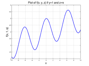
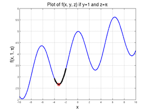
We will assume that two of the three variables (\(y\) and \(z\)) are known and that we want to find \(x\) given those values. We will further assume that \(y=1\) and \(z=\pi\). A graph of this function for values of \(x\) between -10 and 10 is shown at right.
Function on the Fly
If you only want to solve this problem once, and the calculation only requires one line of code, the process with the least "overhead" involves creating the function on the fly inside the fminbnd command. All you have to do is put your expression in for the FUNCTION_THING, making sure the DUMMY_VAR is appropriately used. You will also need to specify the boundary values.
The line:
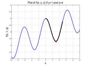
[xValue, fValue] = fminbnd(@(xDummy) xDummy/10 + cos(xDummy) + sin(1) + pi, 0, 5)
will produce
xValue =
   3.0414e+00
fValue =
   3.2922e+00
which has found the local minimum between \(x=0\) and \(x=5\).
Running the code:
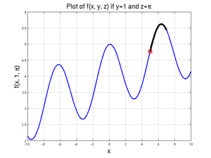
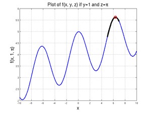
[xValue, fValue] = fminbnd(@(xDummy) xDummy/10 + cos(xDummy) + sin(1) + pi, 5, 7)
will produce
xValue =
   5.0000e+00
fValue =
   4.7668e+00
since, for \(x\) values between 5 and 7, there is no local minimum. The value of the function at 5 is less than the value of the function at 7, so the 5 is returned.
Finally, for
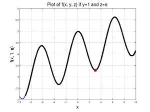
[xValue, fValue] = fminbnd(@(xDummy) xDummy/10 + cos(xDummy) + sin(1) + pi, -9, 10)
MATLAB returns:
xValue =
   3.0414e+00
fValue =
   3.2922e+00
Note that this is not actually the "minimum" minimum - that would be at \(x=-3.2418\), where the function is 2.6639, as given by
[xValue, fValue] = fminbnd(@(xDummy) xDummy/10 + cos(xDummy) + sin(1) + pi, -4, -2)
Furthermore, the actual minimum value of the function over the domain from -9 to 10 is given at \(x=-9\), where \(f=2.1719\); since MATLAB was able to find at least one local minimum, however, it did not check the boundary values.
A slightly "longer" version of this would have you pre-define the \(y\) and \(z\) variables first, then use the variables in the function definition: expression in for the FUNCTION_THING, making sure the DUMMY_VAR is appropriately used. The line:
y = 1;
z = pi;
[xValue, fValue] = fminbnd(@(xDummy) xDummy/10 + cos(xDummy) + sin(y) + z, -4, -2)
This works the same as the last example above - recall that when anonymous functions are created, they can take "snapshots" of the workspace. In the case above, the FUNCTION_THING is able to "see" what the variables y and z contain.
Pre-Defined Functions
If you want to solve the same problem multiple times, perhaps by altering initial guesses or altering one or more of the constant parameters in the function, you should first define the function. If the expression can be calculated all on one line, you may choose to use a variable with an anonymous function - for example:
MyFun = @(xa, ya, za) xa/10 + cos(xa) + sin(ya) + za
On the other hand, if the expression is more complicated or if you just want to put it in a .m file, you can certainly do that as well. For example, instead of the MyFun variable above, you could write a MyFun.m file containing:
function out = MyFun(xb, yb, zb)
out = xb/10 + cos(xb) + sin(yb) + zb;
In either case, you would use fminbnd by properly building the FUNCTION_THING using the name of the function. As in the previous example, you can hard-code the values for the \(x\) and \(y\) values:
[xValue, fValue] = fminbnd(@(xDummy) MyFun(xDummy, 1, pi), -4, 2)
or you can use variables to transmit the information:
y = 1;
z = pi;
[xValue, fValue] = fminbnd(@(xDummy) MyFun(xDummy, y, z), -4, 2)
In any event, note again that the FUNCTION_THING only has one unknown, and that unknown is named as the DUMMY_VAR.
Single-Variable Anonymous Functions
For single-variable anonymous functions, there is a slightly simpler way to run fminbnd - all you need to do is give the name of the variable to FUNCTION_THING rather than setting up the DUMMY_VAR. For example, to find the minimum value of \(x^2-\cos(x)\) on the domain from \(x\) going from -2 to 3, you can set up an anonymous function for it as:
MyAnonCalc = @(x) x.^2-cos(x)
and then solve with:
[xValue, fValue] = fminbnd(MyAnonCalc, -2, 3)
to get
xValue =
  -4.5124e-07
fValue =
  -1.0000e+00
Single-Variable Built-in Functions and .m Functions
The following method works for both built-in single-input functions and .m file single-input functions (i.e. not variables containing anonymous functions). The first argument is the name of the function in single quotes and the second argument is the initial guess or initial bracket for the one variable of the function. For example, to find the minimum value of \(\cos(x)\) for the domain of \(x\) going from 0 to 4, you can type
[xValue, fValue] = fminbnd('cos', 0, 4)
and get
xValue =
   3.1416e+00
fValue =
  -1.0000e+00
If you have a .m file function of one variable, the process is the same. For example, to find the minimum value of \(y=x^2-\cos(x)\) on a domain from -2 to 3, you could first create a .m file called MyCalc.m with:
function out = MyCalc(in)
out = in.^2 - cos(in);
then use fminbnd:
[xValue, fValue] = fminbnd('MyCalc', -2, 3)
and get
xValue =
  -4.5124e-07
fValue =
  -1.0000e+00
Finding Maximum Values
There is no fmaxbnd command. Conveniently, all you need to do to figure out the value and location of the maximum values would be to give fminbnd your function multiplied by -1. The only problem here is that the value of the function fminbnd returns will be the opposite of what you want. For example:
[xValue, fValueSignWrong] = fminbnd(@(xDummy) -(xDummy/10 + cos(xDummy) + sin(1) + pi), 5, 7)
will return
xValue =
   6.3834e+00
fValueSignWrong =
  -5.6164e+00
in order to get the actual value of the function at a maximum, you would need to re-run the calculation or just create a new variable that is equal to -1 multiplied by the function value MATLAB gave:
[xValue, fValueSignWrong] = fminbnd(@(xDummy) -(xDummy/10 + cos(xDummy) + sin(1) + pi), 5, 7)
fValue = -1*fValueSignWrong
to get
xValue =
   6.3834e+00
fValueSignWrong =
  -5.6164e+00
fValue =
   5.6164e+00
Where the Mins Are
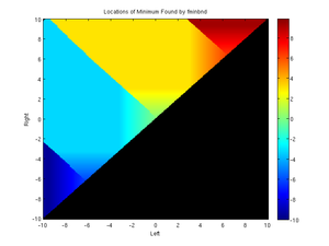
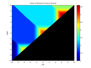
As noted above, if you give MATLAB a domain with multiple local minima, it will not always find the most-minimum minima; here are two graphs showing 19,900 runs of fminbnd with different boundaries. The x axis represents the left boundary and the y axis represents the right boundary.
The black regoins indicate left and right values that will not work since "Right" would be to the left of "Left" there. There are four local minima over the entire domain from -10 to 10. In the left graph, with the locations, these are represented by
- Dark blue: (-9.5250, 2.0356)
- Cyan: (-3.2418, 2.6639)
- Yellow: (3.0414, 3.2922)
- Red: (9.4246, 3.9205)
In the right graph, with the values of the minimum, these are represented by:
- Dark blue: (-9.5250, 2.0356)
- Medium blue: (-3.2418, 2.6639)
- Cyan: (3.0414, 3.2922)
- Green: (9.4246, 3.9205)
For large enough - or well-placed enough - domains, MATALAB will find one of the local minima; if the domain does not span a minimum, it will report back the minimum value at either the left or right boundary. If the domain spans multiple minima, it will report back one of the minima, though not always the minimum one. Notice when the domain is [-10 -4] the dark blue minimum is found, but when the domain is [-10 0], the cyan/medium blue minimum at -3.2418 is found -- even though its value (2.6639) is greater than the value at -9.5250. These graphs show that you need to make sure your domain is large enough to include the minimum you are trying to find but not so large as to include multiple minima.
The code for making these graphs is given in the expandable box here; click the "Expand" link at right.
clear; format short e

MyFun = @(xa, ya, za) xa/10 + cos(xa) + sin(ya) + za
N = 200;
[xl, xr] = meshgrid(linspace(-10, 10, N));
MyMinLoc = zeros(size(xl))-20;
MyMinVal = MyMinLoc;

for k=1:(N-1)
    for l=(k+1):N
        [MyMinLoc(l, k), MyMinVal(l, k)] = ...
            fminbnd(@(xD) MyFun(xD, 1, pi), xl(l, k), xr(l, k));
    end
end

MyMap = jet;

figure(1); clf
%surfc(xl, xr, MyMinLoc)
imagesc(xl(1,:), xr(:,1), MyMinLoc, [-10 10])
set(gca, 'YDir', 'Normal'), xlabel('Left'), ylabel('Right')
title('Locations of Minimum Found by fminbnd')
view(2), shading interp
colormap([0 0 0; MyMap]); BarH = colorbar;
set(BarH, 'YLim', [-10 max(MyMinLoc(:))])
print -dpng -r0 BasinLocations

figure(2); clf
%surfc(xl, xr, MyMinLoc)
imagesc(xl(1,:), xr(:,1), MyMinVal, [2, 5.7])
set(gca, 'YDir', 'Normal'), xlabel('Left'), ylabel('Right')
title('Values of Minimum Found by fminbnd')
view(2), shading interp
colormap([0 0 0; MyMap]); BarH = colorbar;
set(BarH, 'YLim', [2 5.6])
print -dpng -r0 BasinValues
fminsearch
The fminsearch command in MATLAB can be used to find the value of a single vector input of a multivariable function that will minimize the value of the function on some unbounded domain. The command can only find one minimum at a time and can only find minima based on one variable at a time - but that variable can be a vector instead of a single entry.
Most General Case
The following examples show a method that will work regardless of how many input variables your function has or how you define your function - whether it is built-in, a variable containing an anonymous function, an anonymous function generated on the fly, or a .m file function. The paradigm is:
[INDEP_AT_MIN, FUNCTION_MIN] = fminsearch(@(DUMMY_VAR) FUNCTION_THING, INIT_GUESS)
where
- INDEP_AT_MIN is the calculated value of the requested variable when the function is at a minimum in the domain
- FUNCTION_MIN is the minimum value of the function at the INDEP_AT_MIN location
- DUMMY_VAR is the variable you want to use in this FUNCTION_THING to indicate which of the various inputs
fminbndis allowed to alter - FUNCTION_THING can be a built-in function, the name of an anonymous function, the name of a .m file function, or a calculation - whatever it is that you are trying to minimize; note that DUMMY_VAR must appear somewhere in this expression for
fminbndto be able to do anything - INIT_GUESS represents an initial guess for where the minimum value is on the surface. There need to be as many values in the initial guess as there are entries in the dummy variable.
Examples
One Value
If you want to find the location of the minimum of some function \(f(x)\) where \(x\) is a single value (a scalar), all you need is a function and an initial guess. For example, to find the minimum of:
you can run:
f1 = @(x) (x+3).*(x).*(x-1).*(x-3);
[xval, fval] = fminsearch(@(xDummy) f1(xDummy), 0)
and MATLAB will find a minimum of \(f(-2.0234)=-30.01\). Note, however, if you make an initial guess of 1:
[xval2, fval2] = fminsearch(@(xDummy) f1(xDummy), 1)
will return the local - but not global - minimum of \(f(2.2873)=-11.10\). Since there is no way to force fminsearch to find a minimum within a particular set of boundaries, either you should use fminbnd if you only have one parameter or you should be extremely careful in picking your initial conditions. The code below demonstrates that MATLAB finds different locations and values for the minimum depending on initial condition:
clear;
f1 = @(x) (x+3).*(x).*(x-1).*(x-3);
xinit = linspace(-40, 40, 1000);
for k = 1:length(xinit)
    [xval(k), fval(k)] = fminsearch(@(xDummy) f1(xDummy), xinit(k));
end

figure(1); clf
plot(xinit, xval)
xlabel('Initial x'), ylabel('Final x')

figure(2); clf
plot(xinit(fval>-20), f1(xinit(fval>-20)), 'b.', ...
     xinit(fval<-20), f1(xinit(fval<-20)), 'r.')
legend('Basin for min near -11', 'Basin for min of near -30', 'location', 'best')
Multiple Value Vector
Imagine if you were to want to find the minimum of some function
which has a discernible minimum at (1, 2); you could use:
[rval, fval] = fminsearch(@(rDummy) (rDummy(1)-1).^2+(rDummy(2)-2).^2, [0 0])
to have MATLAB start at the origin and find the value of the vector rDummy that has the x and y coordinate in it.
Since this function only has one minimum, MATLAB should be able to find it as long as the initial guess is somewhat reasonable.
Questions
Post your questions by editing the discussion page of this article. Edit the page, then scroll to the bottom and add a question by putting in the characters *{{Q}}, followed by your question and finally your signature (with four tildes, i.e. ~~~~). Using the {{Q}} will automatically put the page in the category of pages with questions - other editors hoping to help out can then go to that category page to see where the questions are. See the page for Template:Q for details and examples.
