Difference between revisions of "MATLAB:Iterative Structures"
| (7 intermediate revisions by the same user not shown) | |||
| Line 1: | Line 1: | ||
| − | + | Often in solving engineering problems you will want a program to run pieces of code several times with slightly - or possibly vastly - different parameters. The number of times to run the code may depend on some logical expression or on the number of columns in a particular matrix. For these, you will use iterative structures. | |
| + | |||
| + | == Indexing Items == | ||
| + | While using a loop, you may want to access certain elements of matrices and vectors within that loop. To do this, you will need a variable that holds on to the index number you want to access. There are two fundamentally different ways to create this variable: using the loop scanning variable itself as in index it appropriate, or creating an external counter. | ||
| + | |||
| + | === Scanner Variable === | ||
| + | If you have a loop that is meant to go through a pre-determined number of iterations, and you have set up a loop counter to count the iteration you are on: | ||
| + | <source lang="matlab"> | ||
| + | for K=1:12 | ||
| + | % Code | ||
| + | end | ||
| + | </source> | ||
| + | you can use the scanning variable as the indexing variable. For instance, to obtain twelve different values from a user, you can use the following code: | ||
| + | <source lang="matlab"> | ||
| + | Temperatures = []; | ||
| + | for K=1:12 | ||
| + | Temperatures(K) = input('Enter a temperature: '); | ||
| + | end | ||
| + | </source> | ||
| + | and the fact that K takes on the values of 1, 2, 3, etc., will work as your index variable. The Temperatures variable will end up as a 1 x 12 matrix with the values the users gave you. | ||
| + | |||
| + | === External Variable === | ||
| + | Sometimes, you will not have an integer-based scanning variable - or you may not have a scanning variable at all (example: while loops). For those, you may have to start an external counter. For example, if you want to store temperature inputs so long as the temperatures entered are non-negative, you could write: | ||
| + | <source lang="matlab"> | ||
| + | NumTemps = 0; | ||
| + | Temperatures = []; % starts off empty | ||
| + | TempInput = input('Enter a temperature (negative to stop): '); | ||
| + | while TempInput>=0 | ||
| + | NumTemps = NumTemps + 1; | ||
| + | Temperatures(NumTemps) = TempInput; | ||
| + | TempInput = input('Enter a temperature (negative to stop): '); | ||
| + | end | ||
| + | </source> | ||
| + | At the end of this code, NumTemps will be a value that indicates how many entries there are in Temperatures, and Temperatures will be a 1 x NumTemps matrix of temperature values. | ||
| + | |||
| + | == Initializing Large Vectors == | ||
| + | One of the dangers in MATLAB's ability to automatically resize a vector is the amount of time it actually takes to do that. | ||
| + | |||
| + | === Iterative Resizing === | ||
| + | Consider the following: | ||
| + | <source lang="matlab"> | ||
| + | clear | ||
| + | tic | ||
| + | y0 = 0; | ||
| + | v0 = 5; | ||
| + | a = -9.81; | ||
| + | NP = 10; | ||
| + | t = linspace(0, 5, NP) | ||
| + | for k=1:NP | ||
| + | y(k) = y0 + v0*t(k) + 0.5*a*t(k).^2; | ||
| + | end | ||
| + | toc | ||
| + | </source> | ||
| + | This code takes, on average, 36 microseconds to run. If NP is increased to 100, the average time to complete goes up to about 150 microseconds. NP of 1000 increases the time to 2.25 ms. And NP of 100000 increases the time to over 10 s! The graph below shows, on a log scale, time to complete as a function of NP: | ||
| + | <center> | ||
| + | [[Image:NoInitPlot.png]] | ||
| + | </center> | ||
| + | |||
| + | Clearly, this becomes a major problem as the number of points increases. | ||
| + | |||
| + | === Initialized === | ||
| + | Remarkably, adding a single line completely changes the timing of the program. The following program: | ||
| + | <source lang="matlab"> | ||
| + | clear | ||
| + | tic | ||
| + | y0 = 0; | ||
| + | v0 = 5; | ||
| + | a = -9.81; | ||
| + | NP = 10; | ||
| + | t = linspace(0, 5, NP) | ||
| + | y = t*0; % here's the only thing that changed!!! | ||
| + | for k=1:NP | ||
| + | y(k) = y0 + v0*t(k) + 0.5*a*t(k).^2; | ||
| + | end | ||
| + | toc | ||
| + | </source> | ||
| + | |||
| + | generates the following time vs. NP graph: | ||
| + | <center> | ||
| + | [[Image:InitPlot.png]] | ||
| + | </center> | ||
| + | which indicates a reduction, by three orders of magnitude, of the run time. And all that was done was creating a vector y of the appropriate size '''before''' running the loop, rather than continuously changing the vector size inside the loop. | ||
| + | |||
| + | === Vectorized === | ||
| + | Of course, the fastest version of the code uses MATLAB's ability to vectorize: | ||
| + | <source lang="matlab"> | ||
| + | clear | ||
| + | tic | ||
| + | y0 = 0; | ||
| + | v0 = 5; | ||
| + | a = -9.81; | ||
| + | NP = 10; | ||
| + | t = linspace(0, 5, NP) | ||
| + | y = y0 + v0*t + 0.5*a*t.^2; | ||
| + | toc | ||
| + | </source> | ||
| + | |||
| + | which generates the following time vs. NP graph: | ||
| + | <center> | ||
| + | [[Image:NoLoopPlot.png]] | ||
| + | </center> | ||
| + | |||
| + | == Questions == | ||
| + | {{Questions}} | ||
| + | |||
| + | == External Links == | ||
| + | |||
| + | == References == | ||
| + | <references /> | ||
| + | |||
| + | |||
| + | [[Category:EGR 103]] | ||
Latest revision as of 04:15, 19 September 2016
Often in solving engineering problems you will want a program to run pieces of code several times with slightly - or possibly vastly - different parameters. The number of times to run the code may depend on some logical expression or on the number of columns in a particular matrix. For these, you will use iterative structures.
Contents
Indexing Items
While using a loop, you may want to access certain elements of matrices and vectors within that loop. To do this, you will need a variable that holds on to the index number you want to access. There are two fundamentally different ways to create this variable: using the loop scanning variable itself as in index it appropriate, or creating an external counter.
Scanner Variable
If you have a loop that is meant to go through a pre-determined number of iterations, and you have set up a loop counter to count the iteration you are on:
for K=1:12
    % Code
end
you can use the scanning variable as the indexing variable. For instance, to obtain twelve different values from a user, you can use the following code:
Temperatures = [];
for K=1:12
    Temperatures(K) = input('Enter a temperature: ');
end
and the fact that K takes on the values of 1, 2, 3, etc., will work as your index variable. The Temperatures variable will end up as a 1 x 12 matrix with the values the users gave you.
External Variable
Sometimes, you will not have an integer-based scanning variable - or you may not have a scanning variable at all (example: while loops). For those, you may have to start an external counter. For example, if you want to store temperature inputs so long as the temperatures entered are non-negative, you could write:
NumTemps = 0;
Temperatures = []; % starts off empty
TempInput = input('Enter a temperature (negative to stop): ');
while TempInput>=0
    NumTemps = NumTemps + 1;
    Temperatures(NumTemps) = TempInput;
    TempInput = input('Enter a temperature (negative to stop): ');
end
At the end of this code, NumTemps will be a value that indicates how many entries there are in Temperatures, and Temperatures will be a 1 x NumTemps matrix of temperature values.
Initializing Large Vectors
One of the dangers in MATLAB's ability to automatically resize a vector is the amount of time it actually takes to do that.
Iterative Resizing
Consider the following:
clear
tic
y0 = 0;
v0 = 5;
a  = -9.81;
NP = 10;
t = linspace(0, 5, NP)
for k=1:NP
   y(k) = y0 + v0*t(k) + 0.5*a*t(k).^2;
end
toc
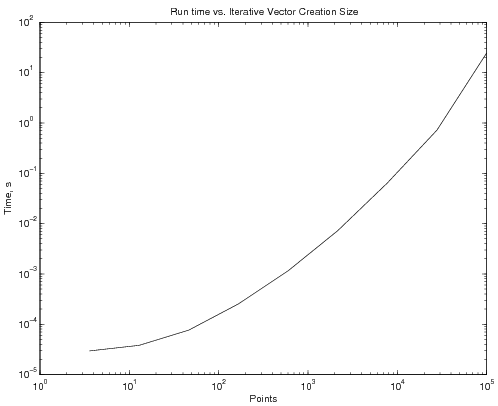
This code takes, on average, 36 microseconds to run. If NP is increased to 100, the average time to complete goes up to about 150 microseconds. NP of 1000 increases the time to 2.25 ms. And NP of 100000 increases the time to over 10 s! The graph below shows, on a log scale, time to complete as a function of NP:
Clearly, this becomes a major problem as the number of points increases.
Initialized
Remarkably, adding a single line completely changes the timing of the program. The following program:
clear
tic
y0 = 0;
v0 = 5;
a  = -9.81;
NP = 10;
t = linspace(0, 5, NP)
y = t*0;     % here's the only thing that changed!!!
for k=1:NP
   y(k) = y0 + v0*t(k) + 0.5*a*t(k).^2;
end
toc
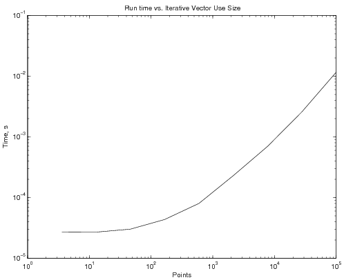
generates the following time vs. NP graph:
which indicates a reduction, by three orders of magnitude, of the run time. And all that was done was creating a vector y of the appropriate size before running the loop, rather than continuously changing the vector size inside the loop.
Vectorized
Of course, the fastest version of the code uses MATLAB's ability to vectorize:
clear
tic
y0 = 0;
v0 = 5;
a  = -9.81;
NP = 10;
t = linspace(0, 5, NP)
y = y0 + v0*t + 0.5*a*t.^2;
toc
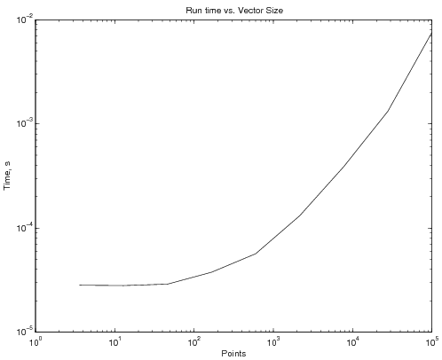
which generates the following time vs. NP graph:
Questions
Post your questions by editing the discussion page of this article. Edit the page, then scroll to the bottom and add a question by putting in the characters *{{Q}}, followed by your question and finally your signature (with four tildes, i.e. ~~~~). Using the {{Q}} will automatically put the page in the category of pages with questions - other editors hoping to help out can then go to that category page to see where the questions are. See the page for Template:Q for details and examples.


