Difference between revisions of "Simulink/Tutorials/DiffEq"
m |
|||
| (2 intermediate revisions by the same user not shown) | |||
| Line 1: | Line 1: | ||
| − | |||
| − | |||
| − | |||
Simulink is a graphical interface type of programming environment especially useful in control systems modeling and a major tool used in both academia and industry for time dependent simulations of dynamical systems. In order to get acquainted with basic Simulink functionality, this lab will walk through how to program a simple second order harmonic oscillator with sinusoidal input | Simulink is a graphical interface type of programming environment especially useful in control systems modeling and a major tool used in both academia and industry for time dependent simulations of dynamical systems. In order to get acquainted with basic Simulink functionality, this lab will walk through how to program a simple second order harmonic oscillator with sinusoidal input | ||
<center><math> | <center><math> | ||
| Line 8: | Line 5: | ||
\end{align} | \end{align} | ||
</math></center> | </math></center> | ||
| − | where m is the mass, c represents damping, k is a restoring spring constant from Hooke’s law, F is the magnitude of the input force, and | + | where m is the mass, c represents damping, k is a restoring spring constant from Hooke’s law, F is the magnitude of the input force, and <math>\omega</math> is the frequency of the input. |
== Opening Simulink == | == Opening Simulink == | ||
[[File:SimModTut1.png|thumb|upright=1|Starting window for Simulink]] | [[File:SimModTut1.png|thumb|upright=1|Starting window for Simulink]] | ||
| − | # Open MATLAB and either type "simulink" in the workspace or click on the Simulink icon on the toolbar: | + | # Open MATLAB and either type "simulink" in the workspace or click on the Simulink icon on the toolbar: [[File:SimulinkIcon.png|15px]] This will open the Simulink Library Browser window. The Simulink library is a categorized list of all the blocks available to write your program. |
| − | + | # Next, start a new Simulink model by either clicking on File-New->Model or clicking the New Model icon, which looks like a blank piece of paper. Simulink programs are called models and save as *.mdl. You should see an blank slate that looks like the figure at right. This is an area to drag and drop blocks and connect them together. | |
| − | # Next, | ||
| − | |||
<br clear=all> | <br clear=all> | ||
| Line 23: | Line 18: | ||
[[File:SimModTut4.png|thumb|upright=1|Adding the addder.]] | [[File:SimModTut4.png|thumb|upright=1|Adding the addder.]] | ||
[[File:SimModTut5.png|thumb|upright=1|Model after adding Sine Wave block.]] | [[File:SimModTut5.png|thumb|upright=1|Model after adding Sine Wave block.]] | ||
| − | # From differential equations and past engineering courses, you know that the harmonic oscillator model in the equation above is second order and relates the first and second derivatives of position (velocity and acceleration). | + | # From differential equations and past engineering courses, you know that the harmonic oscillator model in the equation above is second order and relates the first and second derivatives of position (velocity and acceleration). You first need to construct the relationship between these two systems within the model. |
| − | # In the Library Browser window, click on | + | # In the Library Browser window, click on '''Continuous''' on the menu and find the '''Integrator''' block. |
| − | # Drag and drop two of | + | # Drag and drop two '''Integrator''' blocks into your (previously-blank) model, which one block to the right of the other. |
| − | # As you can see, | + | # Connect them by pointing your mouse at the outward-pointing arrow of the leftmost block, holding down the left-mouse button, then dragging until the line hits the inward-pointing arrow of the rightmost block. There should now be a black line between the blocks. |
| − | + | # Next, create "extension" lines for the input of the leftmost block and the output of the rightmost block. To do this, point to the appropriate arrow, hold down the left mouse button, and drag a few inches away from the block. When you let go, you will get ''red'' lines with an arrowhead. This indicates a wire that is not connected on both sides. | |
| − | # The next step is to add the forces together with the | + | # The names of the blocks can be changed by double clicking on their respective titles and typing in a new name. Similarly, double clicking on a line will let you title the line. The first figure at right shows the model after these processes are complete. |
| − | # Since the external forcing term in the differential equation is <math>F\sin\left(\omega t\right)</math>, all we need to do is create a sinusoidal input with amplitude F. Since Simulink is designed for the type of modeling | + | # As you can see, Simulink will route the acceleration signal through two integrations to derive position. You are now in position to manipulate acceleration, velocity, and position signals as desired by connecting other blocks to them. In the modeling equation, the damping force <math>c\dot{x}</math>and spring force <math>kx</math> can be modeled by routing the velocity and position through '''Gain''' blocks. |
| + | # Back in the Library Browser, select the '''Math Operations''' Library and find the '''Gain''' block. Drag two gain blocks into the workspace, flip them (an option found by right clicking on the block and selecting format), re-label, and connect the signals. An example of this configuration is in the second figure at right. As with nearly all Simulink blocks, you can change parameters by double clicking on the respective block. Since the gain is simply a multiplier, you can put any number or variable previously defined in the MATLAB workspace). | ||
| + | # The next step is to add the damping and spring forces together with the '''Sum'' block (also in '''Math Operations'''). The '''Sum''' block defaults to two inputs, but it can changed to as many as you want by double clicking and including another “+” or “-”. Since we will be modeling acceleration, the modeling equation can be rearranged as <center><math>\begin{align}m\frac{d^2x}{dt^2}=F\sin\left(\omega t\right)-c\frac{dx}{dt}-kx\end{align}</math></center>so you will need one positive input and two negative ones. Replace the code in the '''List of signs''' with "|+--"<br>Also note that the block can be enlarged after one click and resizing as if it were a picture. You can also make the summation block rectangular by double clicking and selecting the icon shape options. The model, after attaching the feedback loops to the sum block, is the third figure at right. | ||
| + | # Since the external forcing term in the differential equation is <math>F\sin\left(\omega t\right)</math>, all we need to do is create a sinusoidal input with amplitude F. Since Simulink is designed for the type of modeling you are doing, you can see the many input options for dynamic systems under the appropriately named '''Sources''' choice in the Library Browser menu. Drag and drop a '''Sine Wave''' block and adjust the parameters by double clicking on it. Note the equation used — your amplitude is F and frequency is <math>\omega</math>. | ||
# Finally, recall that acceleration is force divided by mass, so the acceleration can be isolated as:<center><math> | # Finally, recall that acceleration is force divided by mass, so the acceleration can be isolated as:<center><math> | ||
\begin{align} | \begin{align} | ||
| Line 35: | Line 33: | ||
t\right)-c\frac{dx}{dt}-kx\right) | t\right)-c\frac{dx}{dt}-kx\right) | ||
\end{align} | \end{align} | ||
| − | </math></center>This change is reflected in the last figure at right above by the Netwon’s Second Law (N2L) gain adjustment placed between the | + | </math></center>This change is reflected in the last figure at right above by the Netwon’s Second Law (N2L) gain adjustment placed between the '''Sum''' block and the first '''Integrator''' block. You will need to first delete the wire going from the '''Sum''' block to the first '''Integrator''', then drag in a new '''Gain''' block, then finally make the appropriate connections. |
<br clear=all> | <br clear=all> | ||
== Viewing the outputs == | == Viewing the outputs == | ||
[[File:SimModTut6.png|thumb|upright=1|Model with scope.]] | [[File:SimModTut6.png|thumb|upright=1|Model with scope.]] | ||
| − | # Within the | + | # Within the '''Sinks''' category in the Library Browser there are several options for viewing data. One very useful way is with the '''Scope''' block. All you have to do is connect a display to any signal and Simulink will record the output in a graphical display that can be viewed by double clicking. |
| − | # You can either connect a separate | + | # You can either connect a separate '''Scope''' to any signal you want or have multiple signals route to one '''Scope''' block by double clicking on the '''Scope''', clicking on the parameters icon (second from the left, next to the standard print icon) and changing the number of axes. If running a long time simulation, you might want to go into the data history tab and de-select the Limit data points option. Caution: sometimes too many '''Scopes''' in a very large and complex simulation can slow down the simulation. |
| − | # | + | # You’re done! Select any numerical value you like for k, m, c, F, and <math>\omega</math> and simulate by clicking on the play button. You can adjust the simulation time by changing the value next to the stop button (the simulation time is in seconds). |
# Upon completing the simulation, click on the binoculars button in the scope to normalize all graphs so that all ranges of the data can be viewed. | # Upon completing the simulation, click on the binoculars button in the scope to normalize all graphs so that all ranges of the data can be viewed. | ||
| Line 53: | Line 51: | ||
== References == | == References == | ||
| + | * ''Note: '' This tutorial is taken from the Spring, 2010 printing of "ME125 Laboratory Exercise 1: Data Acquisition, Aliasing and Introduction to SIMULINK Modeling," part of a series of lab assignments written by Robert Clark, Michael R. Gustafson II, Patrick McGuire, Dejan Milutinovic, Monica Rivera, and Milan Simonovic. This tutorial focuses specifically on the introduction to Simulink modeling. Updates as evidenced by this document's history, clickable above. | ||
<references /> | <references /> | ||
{{Protected Class Document}} | {{Protected Class Document}} | ||
| + | [[Category: ME 344]] | ||
Latest revision as of 16:32, 19 February 2013
Simulink is a graphical interface type of programming environment especially useful in control systems modeling and a major tool used in both academia and industry for time dependent simulations of dynamical systems. In order to get acquainted with basic Simulink functionality, this lab will walk through how to program a simple second order harmonic oscillator with sinusoidal input
where m is the mass, c represents damping, k is a restoring spring constant from Hooke’s law, F is the magnitude of the input force, and \(\omega\) is the frequency of the input.
Contents
Opening Simulink
- Open MATLAB and either type "simulink" in the workspace or click on the Simulink icon on the toolbar:
 This will open the Simulink Library Browser window. The Simulink library is a categorized list of all the blocks available to write your program.
 - Next, start a new Simulink model by either clicking on File-New->Model or clicking the New Model icon, which looks like a blank piece of paper. Simulink programs are called models and save as *.mdl. You should see an blank slate that looks like the figure at right. This is an area to drag and drop blocks and connect them together.
Generating a model for the harmonic oscillator
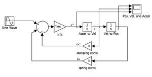
- From differential equations and past engineering courses, you know that the harmonic oscillator model in the equation above is second order and relates the first and second derivatives of position (velocity and acceleration). You first need to construct the relationship between these two systems within the model.
- In the Library Browser window, click on Continuous on the menu and find the Integrator block.
- Drag and drop two Integrator blocks into your (previously-blank) model, which one block to the right of the other.
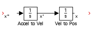
- Connect them by pointing your mouse at the outward-pointing arrow of the leftmost block, holding down the left-mouse button, then dragging until the line hits the inward-pointing arrow of the rightmost block. There should now be a black line between the blocks.
- Next, create "extension" lines for the input of the leftmost block and the output of the rightmost block. To do this, point to the appropriate arrow, hold down the left mouse button, and drag a few inches away from the block. When you let go, you will get red lines with an arrowhead. This indicates a wire that is not connected on both sides.
- The names of the blocks can be changed by double clicking on their respective titles and typing in a new name. Similarly, double clicking on a line will let you title the line. The first figure at right shows the model after these processes are complete.
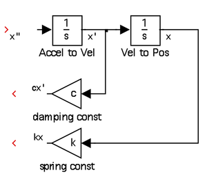
- As you can see, Simulink will route the acceleration signal through two integrations to derive position. You are now in position to manipulate acceleration, velocity, and position signals as desired by connecting other blocks to them. In the modeling equation, the damping force \(c\dot{x}\)and spring force \(kx\) can be modeled by routing the velocity and position through Gain blocks.
- Back in the Library Browser, select the Math Operations Library and find the Gain block. Drag two gain blocks into the workspace, flip them (an option found by right clicking on the block and selecting format), re-label, and connect the signals. An example of this configuration is in the second figure at right. As with nearly all Simulink blocks, you can change parameters by double clicking on the respective block. Since the gain is simply a multiplier, you can put any number or variable previously defined in the MATLAB workspace).
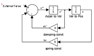
- The next step is to add the damping and spring forces together with the Sum block (also in Math Operations'). The Sum block defaults to two inputs, but it can changed to as many as you want by double clicking and including another “+” or “-”. Since we will be modeling acceleration, the modeling equation can be rearranged as
\(\begin{align}m\frac{d^2x}{dt^2}=F\sin\left(\omega t\right)-c\frac{dx}{dt}-kx\end{align}\) so you will need one positive input and two negative ones. Replace the code in the List of signs with "|+--"
Also note that the block can be enlarged after one click and resizing as if it were a picture. You can also make the summation block rectangular by double clicking and selecting the icon shape options. The model, after attaching the feedback loops to the sum block, is the third figure at right. - Since the external forcing term in the differential equation is \(F\sin\left(\omega t\right)\), all we need to do is create a sinusoidal input with amplitude F. Since Simulink is designed for the type of modeling you are doing, you can see the many input options for dynamic systems under the appropriately named Sources choice in the Library Browser menu. Drag and drop a Sine Wave block and adjust the parameters by double clicking on it. Note the equation used — your amplitude is F and frequency is \(\omega\).
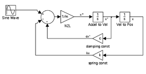
- Finally, recall that acceleration is force divided by mass, so the acceleration can be isolated as:
\( \begin{align} \frac{d^2x}{dt^2}=\frac{1}{m}\left(F\sin\left(\omega t\right)-c\frac{dx}{dt}-kx\right) \end{align} \) This change is reflected in the last figure at right above by the Netwon’s Second Law (N2L) gain adjustment placed between the Sum block and the first Integrator block. You will need to first delete the wire going from the Sum block to the first Integrator, then drag in a new Gain block, then finally make the appropriate connections.
Viewing the outputs
- Within the Sinks category in the Library Browser there are several options for viewing data. One very useful way is with the Scope block. All you have to do is connect a display to any signal and Simulink will record the output in a graphical display that can be viewed by double clicking.
- You can either connect a separate Scope to any signal you want or have multiple signals route to one Scope block by double clicking on the Scope, clicking on the parameters icon (second from the left, next to the standard print icon) and changing the number of axes. If running a long time simulation, you might want to go into the data history tab and de-select the Limit data points option. Caution: sometimes too many Scopes in a very large and complex simulation can slow down the simulation.
- You’re done! Select any numerical value you like for k, m, c, F, and \(\omega\) and simulate by clicking on the play button. You can adjust the simulation time by changing the value next to the stop button (the simulation time is in seconds).
- Upon completing the simulation, click on the binoculars button in the scope to normalize all graphs so that all ranges of the data can be viewed.
Questions
Post your questions by editing the discussion page of this article. Edit the page, then scroll to the bottom and add a question by putting in the characters *{{Q}}, followed by your question and finally your signature (with four tildes, i.e. ~~~~). Using the {{Q}} will automatically put the page in the category of pages with questions - other editors hoping to help out can then go to that category page to see where the questions are. See the page for Template:Q for details and examples.
External Links
References
- Note: This tutorial is taken from the Spring, 2010 printing of "ME125 Laboratory Exercise 1: Data Acquisition, Aliasing and Introduction to SIMULINK Modeling," part of a series of lab assignments written by Robert Clark, Michael R. Gustafson II, Patrick McGuire, Dejan Milutinovic, Monica Rivera, and Milan Simonovic. This tutorial focuses specifically on the introduction to Simulink modeling. Updates as evidenced by this document's history, clickable above.

