Sandbox:Sloth
Jump to navigation
Jump to search
Contents
Edits to directions
Getting Started
- You can get the zip file at the Sunfounder Web Site. Note that site will generally have the latest and greatest version of the instructions. The information on this page was written using a version of the instructions that shipped in Spring 2019.
- Once the zip file downloads, open the file and the 7zip program should come up.
- Click on the DIY 4-DOF Robot Kit - Sloth folder (it should be the only thing in the 7zip window).
- Click on the Extract button at the top pf the window.
- When the "Copy" window opens, click on the button with three dots in it to the right of the path. This should bring up a "Browse for Folder" window.
- Scroll to the top of the "Browse for Folder" window and select Desktop then click the OK button. This should take you back to the "Copy" window.
- Click the OK button in the "Copy" window.
- The DIY 4-DOF Robot Kit - Sloth folder should now be on your desktop. Later, this will simply be called the "Sloth" folder.
Install Arduino IDE
- No changes
Install the Driver
- The Driver folder is in the "Sloth" folder, which should be on the desktop. Open the "Sloth" folder, then the "Driver" folder.
- Double-click the PL2303_Prolific_DriverInstaller_v1180B link to bring up 7zip
- Click the extract icon
- Take note of where the zip file gets extracted - this will be called the "Driver" folder - it is by default the "Driver" folder in the "Sloth" folder
- Once the file is extracted, you should see an application called PL2303_DriverInstaller_v1180_20170406 in the "Driver" folder - double-click the PL2303_DriverInstaller_v1180_20170406 file to run the installer; accept any defaults during installation.
Add libraries
- First run Arduino by either typing Arduino into Cortana and clicking the resulting app or by going into the Windows menu and selecting Arduino
- Follow the instructions in the booklet
- Note you will be warned if the library has already been installed - this doesn't cause problems.
Test for Servos and Ultrasonic Module
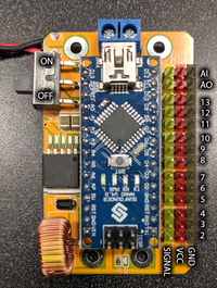
- Note: For the control board, if you look at the bottom figure on p. 9 where the USB cable is up and the power cable is left, there are several groups of three pins each on the right side of the board.
- The first pin (left-most pin) in each group is the signal pin - generally, the yellow or orange wire of a servo goes here.
- The middle pin is the VCC, or high voltage, pin - generally, the red wire of a servo goes here.
- The last pin (right-most pin) is the GND, or ground, pin - generally, the brown wire of a servo goes here.
- The bottom group of three pins is for Channel 2; the channel increases as you go up to Channel 13, which is two from the top. The next-to-the-top is the AO (analog out) channel and the top is the AI (analog in) channel.
- Servo test
- Physical test
- Preparing the servo means using the small screw from the servo connections bag to attach the 1-sided horn to the servo.
- Software test
- Test code is in the Sloth Directory under Code/Test_Robot
- Start the Arduino sketch editor program and load the test code. Without connecting the Ardiuno's USB cable to the computer, in the sketch editor go to Tools->Port and write down which COM ports are showing. Click somewhere outside the menu to make it go away. Now plug the Arduino's USB cable in. Go back to Tools->Port and select whichever COM port wasn't there before.
- Be sure to go to Tools->Board and select Arduino/Nano
- Also go to Tools->Procesor and select "ATmega328P (Old Bootloader)"
- The brown wire on the servo connection will be closest to the edge of the control board; the yellow wire will be closes to the nano; in the figure on p. 11 of the booklet, the yellow wires are to the left and the brown wires are to the right.
- From the perspective of figure on p. 11 of the booket, Pin12 is the fourth header from the top. Once the connections are made, going from top to bottom, there will be three empty headers, followed by servos on channels 12 through 9, followed by 7 empty headers.
- The power switch on the driver board should start in the position closest to the battery connection (up in the figure). When the instructions say "press the power button," they really mean flip the switch on the control board (putting the switch in the down position will allow the 9V batter to drive the servos).
- Note that the servos may not be accurately by sweeping through 180 degrees
- When you are done with the test, you will want to turn the servos off; to do that:
- In Arduino, go to File->Examples->01.Basics->BareMinimum
- Upload that sketch; once finished, the servos should stop moving.
- Physical test
- Ultrasonic test
- Typo: on the top of p. 12 in the first line, it should say that TRIGGER_PIN is **4** and ECHO_PIN is **3**
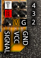
- In connecting the sensor to the board, from the perspective of the figure above (not the one on p. 12):
- Black wire is GND -- this will be the bottom right pin of the control board (GND for channel 2)
- Brown wire is VCC -- this will be the pin just left of that (VCC for channel 2 - rare case where VCC is brown)
- Red wire is Echo -- this will be the left pin one row up from the bottom (signal for channel 3)
- White wire is Trig -- this will be the left pin two rows up from the bottom (signal for channel 4)
- "disable the SERVO and activate the ULTRASONIC" means adding // to the start of line 16 and deleting the // from the start of line 16. In Arduino, // starts a comment. Note - if you run the test and the servos are moving and the ping distance is only updating every second or so, you likely forgot to disable SERVO - check your program and upload it again.
- The serial monitor is in Tools->Serial Monitor
- The batter needs to be connected and the board needs to be turned on (switch in the down position)
- When done, once again go to File->Examples->01.Basics->BareMinimum; upload this sketch; then turn the battery off.
Assembly
- Head Assembly
- Be careful! The parts are very small - lay some paper on the lab bench or the floor and work near the middle of the paper so you can see any pieces you may drop.
- The standoffs will be installed over the four small round holes near the middle of the head. The ones near the sensor are very close together; the ones furthest from the sensor are separated by the large oval. The easiest thing to do here is push the screw through the hole, hold it in place with one hand, and then screw the standoff onto it. Do not use the screwdriver for these.
- Electrical Module Assembly
- The easiest way to do the first step (connecting circuit board) is to put all four screws in, then carefully place the assembly on top of the standoffs. Note that the screwdriver is too small to really tighten these screws so do the best you can without stripping the screws or damaging the screwdriver.
- The easiest way to do the second part (longer standoffs) is to push the screw through the hole, hold it in place with one hand, and then screw the standoff onto it.
- Servo Assembly
- The servo fires should be pointing to the rounder end of the No. 2 board
- When attaching the two boards together, the flatter part will be under the ultrasonic sensor and the rounder end - where the wires from the servos are - will be under the USB connector on the nano.
- Page 16 is not in the smartest order! Do the bottom step of assembling the 1-arm rocker to the 4-board first, then go back to the top of the page and do those three steps.
- When connecting the 4th and 5th boards, be sure that you put the screw through the lower small hole on board 5, then a small hole on board 4, then make sure the larger part of the nut is inboard (pressing on board 4). Also, whichever small hole you used on the first board 5, use the other on the second assembly.
Contents of Box
- Instruction booklet
- Compliance and safety notice
- Structural parts:
- Bottom plate
- Top plate
- Feet (2)
- Motor chassis (2)
- Motor frame (2)
- Fasteners:
- 1.5*5 screw (10)
- 1.4*8 screw (6)
- 2*8 screw (12)
- 3*5 screw (18)
- 3*8 countersunk screw (8)
- 1.4 nut (6)
- 2 nut (12)
- 3 self-locking nut (8)
- 3*8 standoff (4)
- 3*25 standoff (4)
- Electrical:
- servo (4)
- ping (1)
- nano board (1)
- expansion board (1)
- velcro tape (1)
- mini usb cable (1)
- 9V battery connection (1)
- 4-pin cable (1)
- Phillips screwdriver
- Socket wrench (1)
- Included, not explicitly listed in booklet:
- Servo connectors (1, 2, and 4 sided horn) (4)
- Screws with servo connector (sm, med, lrg) (4)
- Not included
- 9V battery

