Singularity Functions
Singularity Functions are a class of functions that - you guessed it - contain singularities. One notation for a singularity function is given as adapted from p. 77 Chapra[1]
where \(x\) is the independent variable and \(n\) and \(x_0\) are constants. Note that this definition is only useful when \(n\geq 0\). Negative values of \(n\) are used to denote the impulse function (when \(n=-1\)) or its derivatives. Also note that it is common to leave the singularity undefined when \(n=0\) and \(x=x_0\). That is to say, a fuller definition of the singularity function might be:
where the delta function \(\delta(x)\) and its derivatives will be defined below.
Contents
Basic Definitions and Derivations
Alternate Names for \(n\geq 0\)
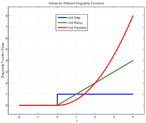
In courses such as ECE 54 and EGR 224, alternate names are given to different non-negative powers of the singularity function. Furthermore, singularity functions are generally written as functions of time rather than space, so:
For the last entry, you may be tempted to ask, "How is that the unit parabola?" The simplest explanation is that the unit ramp is the integral of the unit step, and the unit parabola is the integral of the unit parabola.
Derivation of Unit Impulse Functions
You can also take derivatives of the singularity functions. For \(n>0\), this is quite easy as the unit ramp and above are continuous. The difficulty comes in taking the derivative of the \(<t-a>^0\) case. Mathematically, call the derivative of the unit step function \(\delta(t)\); you can then find
But how large is that infinity? The answer comes in integrating this "delta function" (also known as the "unit impulse function" or just "impulse function"):
and by definition,
meaning
In other words (well...in words) the total area is 0 when integrating between negative infinity and just before 0 and the total area is 1 when integrating between negative infinity and anything positive. That must mean, at exactly \(t=0\), \(\delta(t)\) has an area of 1 while for all other times, it has an area of 0. That is to say,
Variable Transformations for Unit Step and Unit Impulse
Three common transformations of the independent variable (in the examples, \(t\)) are scaling, shifting, and reversing. The following pairs show how scaling (multiplying the independent variable by some positive constant \(a\)), shifting (subtracting some value \(t_0\) from the independent variable), and reversing (multiplying the independent variable by -1) may be written in alternate ways. First, for the unit step function:
Note that a positive time scaling does not have an effect on the unit step function. Also note in the final two cases above that the independent variable is first shifted, then scaled or scaled and reversed.
For the unit impulse function, time scaling is a bit more complex. Fortunately, time reversal is much simpler:
Building a Mystery Signal
Often, singularity functions will be used to build piecewise signals. There are two fundamentally different methods for this.
Logical Masks
Piecewise Constants
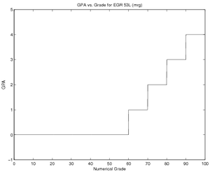
First, singularity functions can be used to create "windows" for each piece of the signal. This method effectively uses step functions to create Logical Masks. For example, the GPA function at right could be defined in terms of Grade \(G\) as:
\( \mbox{GPA}(G)=\left\{ \begin{array}{rl} 4.0, & G\geq 90~~~\\ 3.0, & 80\leq G ~\And~ G<90~~~\\ 2.0, & 70\leq G ~\And~ G<80~~~\\ 1.0, & 60\leq G ~\And~ G<70~~~\\ 0.0, & G<60~~~ \end{array} \right. \)
Each window can be created by taking the difference between two step functions - one that turns "on" at the low end of the grade and one that turns "on" at the high end. For example, the "B" window would be defined, using step functions, as:
This window is 1 when the grade is between 80 and 90 and 0 otherwise (note: using the formal definition of the step function given above, this does cause a bit of uncertainty for people who have grades of exactly 80 or 90.) To get the correct GPA for those grades, simply multiply each window by the appropriate GPA value. The full function would thus be:
Piecewise Functions
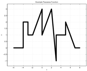
The case above simply had constant values in each window. You can also have piecewise function where the windows have values that are functions of the independent variable - such as the one given at right. The "window" based definition of this signal is:
\( x(t)=\left\{ \begin{array}{rl} 0, & t< -4\\ 2, & -4\leq t < -3\\ 1, & -3\leq t < -2\\ t+3, & -2\leq t < 0\\ t+1, & 0\leq t < 2\\ -4t+11, & 2\leq t < 3\\ 1, & 3\leq t < 5\\ -t+7, & 5\leq t < 7\\ 0, & t\geq 7\\ \end{array} \right. \)
and the signal could therefore be written using nine pieces, each comprised of a produce of a step function or difference of step functions followed by a formula. In this particular case, the number of pieces could be reduced to seven since the signal has no values for times before -4 sec or after 7 sec. This gets a bit messy, however:
Accumulated Differences
Another method for building a signal is to look at how the signal changes at a particular point and multiplying that change by the appropriate step function. This is most useful when the changes are limited to jumps or drops in value and/or changes in slope; more complicated piecewise functions are best done using the logical mask method above.
GPA
To being, revisit the GPA function above. For the accumulated difference method, there must be some point in time before which the signal is 0 - in this case, that point is when the grade is 60. From that point forward, you will accumulate differences by writing the appropriate step function for changes in value or ramp function for changes in slope. The first change is a jump of height 1 when the grade hits 60:
The next change is a jump of height 1 when the grade passes 70. To add this, simply have a unit step function turn on, with the appropriate jump height, at G=70:
The next jumps are at 80 and 90, and each jump has a value of 1, so the final function can be written as:
or, simplifying the fact that the heights are always 1 in this particular case:
Though it is not as clear to a viewer what this means in terms of the function's value at each location, it is certainly simpler than the Piecewise Constants version.
Piecewise Function
For the piece-wise function
\(\begin{align} x(t)=&~(2)*u(t+4)+... ~&\mbox{Change value by +2 at t=-4}\\ ~&~ (-1)*u(t+3)+... ~&\mbox{Change value by -1 at t=-3}\\ ~&~ (1)*r(t+2)+... ~&\mbox{Change slope by +1 at t=-2}\\ ~&~ (-2)*u(t)+... ~&\mbox{Change value by -2 at t=0}\\ ~&~ (-5)*r(t-2)+... ~&\mbox{Change slope by -5 at t=2}\\ ~&~ (4)*r(t-3)+... ~&\mbox{Change slope by +4 at t=3}\\ ~&~ (2)*u(t-3)+... ~&\mbox{Change value by +2 at t=3}\\ ~&~ (-1)*r(t-5)+... ~&\mbox{Change slope by -1 at t=5}\\ ~&~ (1)*u(t-5)+... ~&\mbox{Change value by +1 at t=5}\\ ~&~ (1)*r(t-7)~&\mbox{Change slope by +1 at t=7}\\ \end{align} \)
Note that this version is much easier to convert to a Laplace Transform than the logical masks, specifically because there are no differently-shifted terms.
General Simplification of Integrals
The impulse function and step function, as part of an integrand, may make analysis of the integral simpler through a variety of ways. The following simplifications are broken up into four categories depending on which singularity function is used and whether it is the sole integrand or part of a more complex expression.
Integrand with Impulse Functions Only
As should be clear about, the impulse function, as an integrand, is only non-zero when its argument is exactly zero and that that point, it has an area of 1. These properties help simplify integrals involving only impulse functions:
Impulse Functions as Part of Integrand
Impulse functions as part of an integrand can also lead to simplifications involving more than just impulse functions in the integrand:
Integrand with Step Functions Only
Step Functions as Part of Integrand
Convolution Integral Simplification with Step Function Product as Part of Integrand
The convolution integral
will generate products of step functions in the integrand if both \(x(t)\) and \(h(t)\) are defined using step functions. There are two main ways to get a product of step functions as an integrand - either they are both "pointing" in the same direction or they are pointing in opposite directions.
Same Directions in Integrand
If the step functions are "pointing" in the same direction in \(\tau\) space - that is
the key is to recognize that, for the integrand to be non-zero, you must satisfy the inequalities
You will thus need to determine which of these presents the stricter condition. Then:
which can be re-written using unit step functions as:
Opposite Directions in Integrand
This is the case that most often comes into play during convolution:
where the first step function is right-sided in \(\tau\) and the second function is left-sided. For the integrand to be nonzero,
This clearly indicates the limits on the integral - but it also indicates a restriction on time. That is, for both inequalities to be satisfied,
which gives rise to a unit step function that can be written outside the integral since it is not a function of \(\tau\). Specifically,
Questions
Post your questions by editing the discussion page of this article. Edit the page, then scroll to the bottom and add a question by putting in the characters *{{Q}}, followed by your question and finally your signature (with four tildes, i.e. ~~~~). Using the {{Q}} will automatically put the page in the category of pages with questions - other editors hoping to help out can then go to that category page to see where the questions are. See the page for Template:Q for details and examples.
External Links
References
- ↑ Applied Numerical Methods with MATLAB for Engineers and Scientists, 2/e, Steven C. Chapra


