MATLAB:Ordinary Differential Equations/Examples
The following examples show different ways of setting up and solving initial value problems in MATLAB. It is part of the page on Ordinary Differential Equations in MATLAB.
Contents
Examples
Note - each example began with the Templates provided at this web site. Some comments have been removed from the templates to conserve space while some comments may have been added to provide a clearer explanation of the process for a particular example.
Constant Rate of Change
If the dependent variable has a constant rate of change:
where \(C\) is some constant, you can provide the differential equation
with a function called ConstDiff.m that contains the code:
function dydt = ConstDiff(t, y, C)
% Differential equation for constant growth
% t is time
% y is the state vector
% C contains any required constants
% dydt must be a column vector
dydt = C(1); % or just C since there is only one
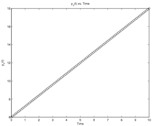
You could calculate answers using this model with the following code
called RunConstDiff.m,
which assumes there are 100 evenly spaced times between 0 and 10, the
initial value of \(y\) is 6, and the rate of change is 1.2:
% Initialize workspace and graph
clear; format short e; figure(1); clf

% Set name of file containing derivatives
DiffFileName = 'ConstDiff';

% Set up time span, initial value(s), and constant(s)
% Note: Variables should be in columns
tspan = linspace(0, 10);
yinit = 6;
C = 1.2;

% Determine if states should be plotted
PlotStates = 1;

%% Under the hood
% Use ODE function of choice to get output times and states
DE = eval(sprintf('@(t, y, C) %s(t,y,C)', DiffFileName))
[tout, yout] = ode45(@(t,y) DE(t,y,C), tspan, yinit);

% Plot results
if PlotStates
    figure(1); clf
    StatePlotter(tout, yout)
end
Time-dependent Rate of Change
If the dependent variable's rate of change is some function of time, this can be easily written using MATLAB. For example, if the differential equation is some quadratic function given as:
then the function providing the values of the derivative may be
written in a file called TimeDiff.m
function dydt = TimeDiff(t, y, C)
% Differential equation for time-based polynomial derivative
% t is time
% y is the state vector
% C contains any required constants
% dydt must be a column vector
dydt = polyval(C, t);
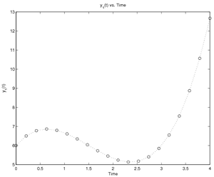
You could calculate answers using this model with the following code
called RunTimeDiff.m,
which assumes there are 20 evenly spaced times between 0 and 4, the
initial value of \(y\) is 6, and the polynomial is defined by the vector
[2 -6 3]:
% Initialize workspace and graph
clear; format short e; figure(1); clf

% Set name of file containing derivatives
DiffFileName = 'TimeDiff';

% Set up time span, initial value(s), and constant(s)
% Note: Variables should be in columns
tspan = linspace(0, 4, 20);
yinit = 6;
C     = [2 -6 3];

% Determine if states should be plotted
PlotStates = 1;

%% Under the hood
% Use ODE function of choice to get output times and states
DE = eval(sprintf('@(t, y, C) %s(t,y,C)', DiffFileName))
[tout, yout] = ode45(@(t,y) DE(t,y,C), tspan, yinit);

% Plot results
if PlotStates
    StatePlotter(tout, yout)
end
Population Growth
For population growth, the rate of change of population is dependent upon the number of people as well as some constant of proportionality:
where \(C\) is again some constant.
In that case, the function may be written in a file called PopDiff.m as follows:
function dydt = PopDiff(t, y, C)
% Differential equation for population growth
% t is time
% y is the state vector
% C contains any required constants
% dydt must be a column vector
dydt = C(1)*y(1); % or just C*y since both are 1x1
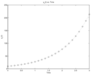
The following code, RunPopDiff.m, will calculate the population for
a span of 3 seconds with 25
points for the population model above with an initial population of 10
and a constant of proportionality of 1.02:
% Initialize workspace and graph
clear; format short e; figure(1); clf

% Set name of file containing derivatives
DiffFileName = 'PopDiff';

% Set up time span, initial value(s), and constant(s)
% Note: Variables should be in columns
tspan = linspace(0, 3, 25);
yinit = 10;
C     = 1.02;

% Determine if states should be plotted
PlotStates = 1;

%% Under the hood
% Use ODE function of choice to get output times and states
DE = eval(sprintf('@(t, y, C) %s(t,y,C)', DiffFileName))
[tout, yout] = ode45(@(t,y) DE(t,y,C), tspan, yinit);

% Plot results
if PlotStates
    StatePlotter(tout, yout)
end
Multiple Variable Models
It is possible to solve multiple-variable systems by making sure the differential function returns values for each of the variables. For instance, in the following system the first variable's rate of change depends only on time while the second is dependent upon both time and the first variable:
The differential file TwoDiff.m for this system will have a 2x1
matrix as the output:
function dydt = TwoDiff(t, y, C)
% Differential equations for two variables
% t is time
% y is the state vector
% C contains any required constants
% dydt must be a column vector
dydt = [...
    C(1)*cos(C(2)*t);...
    C(3)*y(1)+C(4)*t];
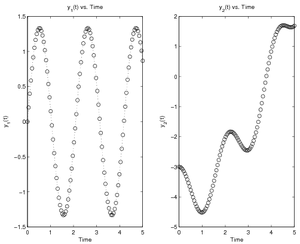
Finally, if you have systems with multiple dependent variables, just be sure to put the initial conditions in a column vector. For example, with the system defined as:
you could use the following script called RunTwoDiff to solve for both
\(y_1\) and \(y_2\) assuming \(y_1\) starts as 0 and \(y_2\) starts at -3:
% Initialize workspace and graph
clear; format short e; figure(1); clf

% Set name of file containing derivatives
DiffFileName = 'TwoDiff';

% Set up time span, initial value(s), and constant(s)
% Note: Variables should be in columns
tspan = linspace(0, 5);
yinit = [0 -3]';
C     = [4 3 -2 0.5];

% Determine if states should be plotted
PlotStates = 1;

%% Under the hood
% Use ODE function of choice to get output times and states
DE = eval(sprintf('@(t, y, C) %s(t,y,C)', DiffFileName))
[tout, yout] = ode45(@(t,y) DE(t,y,C), tspan, yinit);

% Plot results
if PlotStates
    StatePlotter(tout, yout)
end
Higher Order Differential Equations
The system must be written in terms of first-order differential equations only. To solve a system with higher-order derivatives, you will first write a cascading system of simple first-order equations then use them in your differential file. For example, assume you have a system characterized by constant jerk:
The first thing to do is write three first-order differential equations to represent the third-order equation:
Notice how the derivatives cascade so that the constant jerk equation
can now be written as a set of three first-order equations. The
differential file JerkDiff.m would thus be:
function dydt = JerkDiff(t, y, C)
% Differential equations for constant jerk
% t is time
% y is the state vector
% C contains any required constants
% dydt must be a column vector
dydt = [...
     y(2); ...
     y(3);...
     C(1)]; % or just C since there is only one
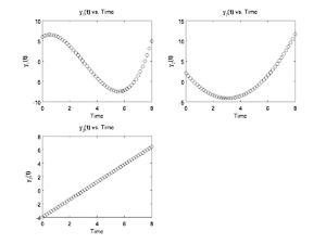
to represent the three equations given above. Note that in this system, \(y_1\) represents the position, \(y_2\) represents the velocity, and \(y_3\) represents the acceleration. This type of cascading system will show up often when modeling equations of motion.
The following script, RunJerkDiff.m, calculates the position,
velocity, and speed over a period of 8 seconds assuming an initial
position of 6, and initial velocity of 2, an initial acceleration of
-4, and a constant jerk of 1.3:
% Set name of file containing derivatives
DiffFileName = 'JerkDiff';

% Set up time span, initial value(s), and constant(s)
% Note: Variables should be in columns
tspan = linspace(0, 8, 50);
yinit = [6 2 -4];
C     = 1.3;

% Determine if states should be plotted
PlotStates = 1;

%% Under the hood
% Use ODE function of choice to get output times and states
DE = eval(sprintf('@(t, y, C) %s(t,y,C)', DiffFileName))
[tout, yout] = ode45(@(t,y) DE(t,y,C), tspan, yinit);

% Plot results
if PlotStates
    StatePlotter(tout, yout)
end
Note in the above that the StatePlotter function is called to plot the states. That code is:
function StatePlotter(Time, States)

StateCount = size(States, 2);

NumCols = ceil(sqrt(StateCount));
NumRows = ceil(StateCount / NumCols);
clf;
for PlotNumber = 1:StateCount
        subplot(NumRows, NumCols, PlotNumber);
        plot(Time, States(:,PlotNumber), 'ko:');
        xlabel('Time');
        ylabel(sprintf('y_{%0.0f}(t)', PlotNumber))
        title(sprintf('y_{%0.0f}(t) vs. Time', PlotNumber));
end
Questions
Post your questions by editing the discussion page of this article. Edit the page, then scroll to the bottom and add a question by putting in the characters *{{Q}}, followed by your question and finally your signature (with four tildes, i.e. ~~~~). Using the {{Q}} will automatically put the page in the category of pages with questions - other editors hoping to help out can then go to that category page to see where the questions are. See the page for Template:Q for details and examples.
